Week 2 - Flow over a Cylinder.
Challenge-2
Aim:- Simulate the flow over a cylinder and explain the phenomenon of Karman vortex street
PART-I
- Simulate the flow with the steady and unsteady case and calculate the Strouhal Number for Re= 100.
PART-II
- Calculate the coefficient of drag and lift over a cylinder by setting the Reynolds number to 10,100,1000,10000 & 100000 with steady solver.
Introduction :-
Von karman vortex shading
In fluid dynamics, a Kármán vortex street (or a von Kármán vortex street) is a repeating pattern of swirling vortices, caused by a process known as vortex shedding, which is responsible for the unsteady separation of flow of a fluid around blunt bodies.
Vortex shading
In fluid dynamics, vortex shedding is an oscillating flow that takes place when a fluid such as air or water flows past a bluff (as opposed to streamlined) body at certain velocities, depending on the size and shape of the body. In this flow, vortices are created at the back of the body and detach periodically from either side of the body forming a Von Kármán vortex street. The fluid flow past the object creates alternating low-pressure vortices on the downstream side of the object. The object will tend to move toward the low-pressure zone.
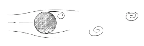
Fig 1 Vortex shading
Reynolds number
Reynolds number is a dimensionless quantity that is used to determine the type of flow pattern as laminar or turbulent while flowing through a pipe.
Which is ratio of inertia force to the viscous force
Reynolds number= inertial force / viscous force
`re=(rho*v*D)/mu`
Importance in practical applications
A vortex is in the process of formation near the top of the cylinder surface. Below and to the right of the first vortex is another vortex which was formed and shed a short period before. Thus, the flow process in the wake of a cylinder or tube involves the formation and shedding of vortices alternately from one side and then the other. This phenomenon is of major importance in engineering design because the alternate formation and shedding of vortices also creates alternating forces, which occur more frequently as the velocity of the flow increases.
When the frequency is in the audible range, a sound can be heard and the body appears to sing. Resonance may occur if the vortex shedding frequency is near the structural-vibration frequency of the body. A dimensionless number, the Strouhal number Sr, is commonly used as a measure of the predominant shedding frequency fs. The definition is
`Strouhal Number=(f*d)/u`
f- vortex shading frequency
d charecterstic length
u flow velocity
Solving and modelling approach :-
Geometry making:-
Using sketch 2D model is created in spaceclaim application of cylinder/ circle of 2m diameter and length and breadth of model 60 and20 m respectively ad the cylinder/ circle is created 40m from left end and middle from top to bottom using pull command surface is created.
Once surface is created close the spaceclaim
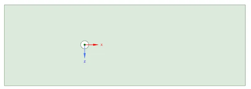
Fig 1 model
Mesh
From workbench launch the mesh application once the file is opened change the element size of mesh to 0.25m and right click on mesh select insert option select method and apply the model by face selection and select method as all triangles method similarly add edge sizzing and inflation in that body fit to make cylinder more circular and create body fit inflation to capture the results more accurately once done generate the mesh once mesh is done.
Name the left edge as inlet by select edge and right edge as outlet and cylinder as cell wall and close the application
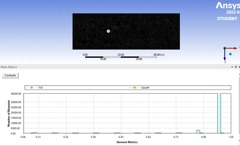
Fig 2 mesh quality of model
Setup
Check for mesh quality once enter into the fluent application then select vicous model ad laminar model in materials create new material to do so select any material which is there and copy those property and give a new name to the copied martial and delete other fluid present in selection drop down
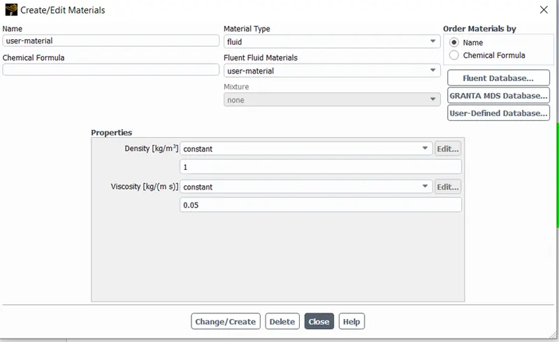
Fig 3 User material property
Boundary condition only inlet velocity is given
Case 1 steady case with Reynolds number 100
Inlet velocity as 2.5m/s
`Re=(rho*v*D)/mu`
Re= 1*2.5*2/0.05=100
In set up select general solver as pressure based , velocity formulation as absolute and time as steady
In solution section remove converge option from residual section
A point is created away from center to 8 m to right side to moniter5 the velocity at that point
Point is created now in definition create report of velocity ant that point , drag coefficient and lift coefficient report and plot are selected as well as create output parameter in solution select simple discretization and to create animation from activity select animation from solution and select the parameter for which the animation is created and initialize the calculation by clicking initialization command and then enter the no of iteration and click on calculate command and wait till calculation done
calculation is done then check animation and click video write from drop down and create the video of the animation to plot Strouhal Number go to result from plot click on fft in that from drop down select Strouhal Number and load the file from the system and plot the graph.
Once all th calculation is done close the fluent and n workbench from parameter section note down the drag, lift coeffient and monitor velocity
Go to result and look at animation and result
results of case 1 steady case
drag coeffient 13.55
lift coeffient 0.416
moniter velocity 1.35
Case 1
Simulate the flow with the steady and calculate the Strouhal Number for Re= 100
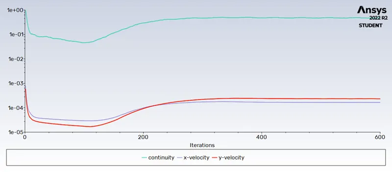
Fig 4 residuel moniter
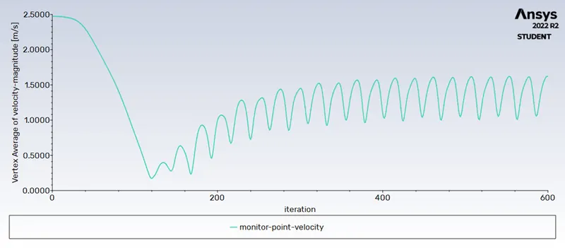
fig 5 moniter velocity plot
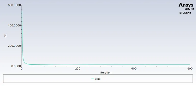
Fig 6 drag coefficent
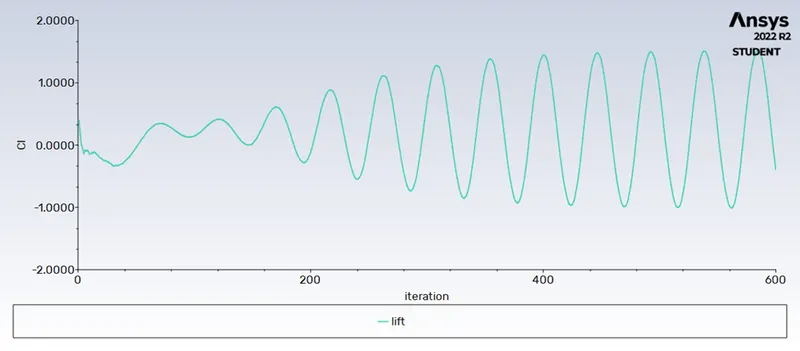
Fig 7 Lift coefficent
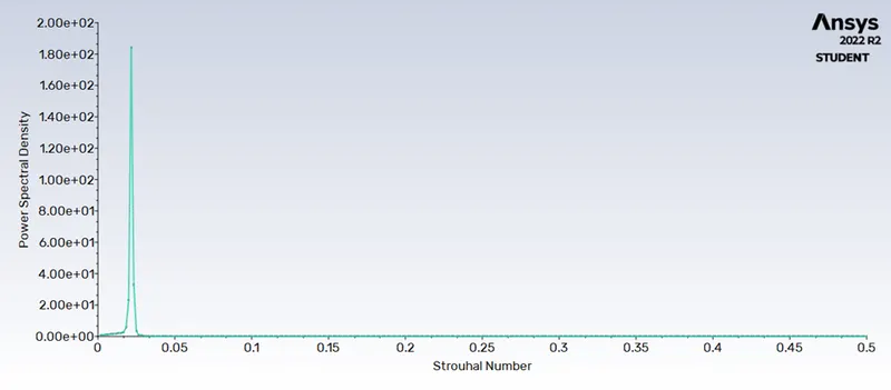
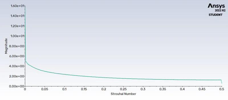
Fig 8 Strouhal Number
Case 2 Unsteady case with Reynolds number 100
Inlet velocity as 2.5m/s
`Re=(rho*v*D)/mu`
Re= 1*2.5*2/0.05=100
In set up select general solver as pressure based, velocity formulation as absolute and time as transient
In solution section remove converge option from residual section
A point is created away from center to 8 m to right side to moniter the velocity at that point
Point is created now in definition create report of velocity ant that point , drag coefficient and lift coefficient report and plot are selected as well as create output parameter in solution select simple discretization and to create animation from activity select animation from solution and select the parameter for which the animation is created and initialize the calculation by clicking initialization command and then enter the no of time step and click on calculate command and wait till calculation done
calculation is done then check animation and click video write from drop down and create the video of the animation to plot Strouhal Number go to result from plot click on fft in that from drop down select Strouhal Number and load the file from the system and plot the graph.
Once all th calculation is done close the fluent and n workbench from parameter section note down the drag, lift coeffient and monitor velocity
Go to result and look at animation and result
results of case 1 unsteady case
drag coeffient 13.466
lift coeffient 0.416
moniter velocity 1.27
Simulate the flow with the unsteady case and calculate the Strouhal Number for Re= 100
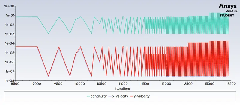
fig 9 residuel moniter
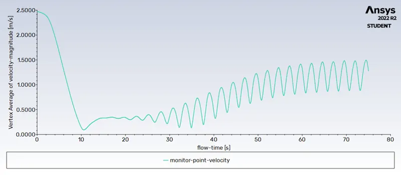
fig 10 moniter velocity
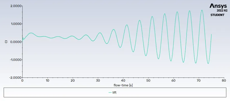
fig 11 lift coeeficent
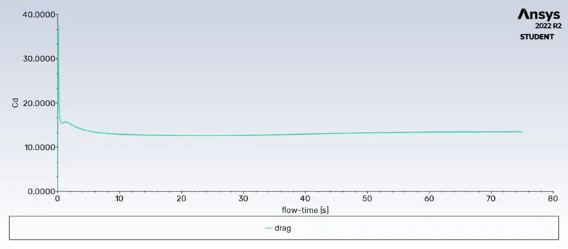
fig 12 drag coeffeficent
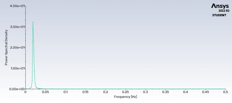
fig 13 Strouhal Number plot
Case 2 Calculate the coefficient of drag and lift over a cylinder
1 Reynolds number = 10
Case 1 steady case with Reynolds number 100
Inlet velocity as 2.5m/s
`Re=(rho*v*D)/mu`
Re= 1*0.25*2/0.05=10
In set up select general solver as pressure based, velocity formulation as absolute and time as steady
In solution section remove converge option from residual section
A point is created away from centre to 8 m to right side to moniter5 the velocity at that point
Point is created now in definition create report of velocity ant that point , drag coefficient and lift coefficient report and plot are selected as well as create output parameter in solution select simple discretization and to create animation from activity select animation from solution and select the parameter for which the animation is created and initialize the calculation by clicking initialization command and then enter the no of iteration and click on calculate command and wait till calculation done
calculation is done then check animation and click video write from drop down and create the video of the animation to plot Strouhal Number go to result from plot click on fft in that from drop down select Strouhal Number and load the file from the system and plot the graph.
Once all the calculation is done close the fluent and n workbench from parameter section note down the drag, lift confident and monitor velocity
Go to result and look at animation and result
results of case 2 steady case Re 10
drag coeffient 0.338
lift coeffient 0.0003937
moniter velocity 0.105 m/s
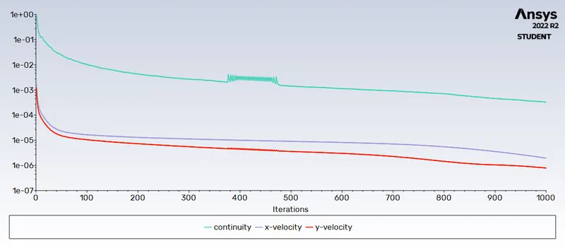
fig 14 residual moniter
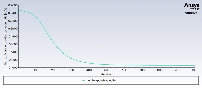
fig 15 velocity monitor
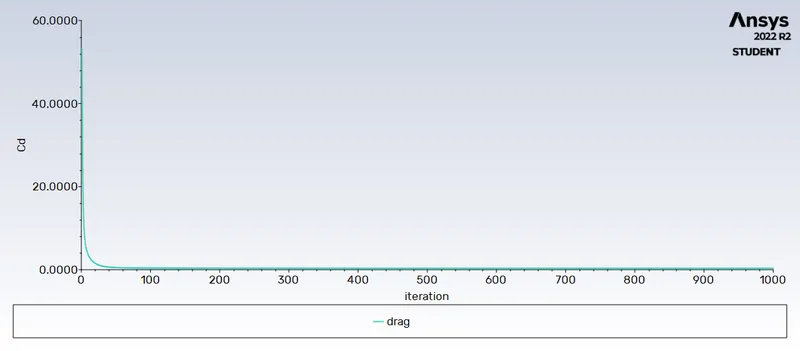
fig 16 drag coefficient
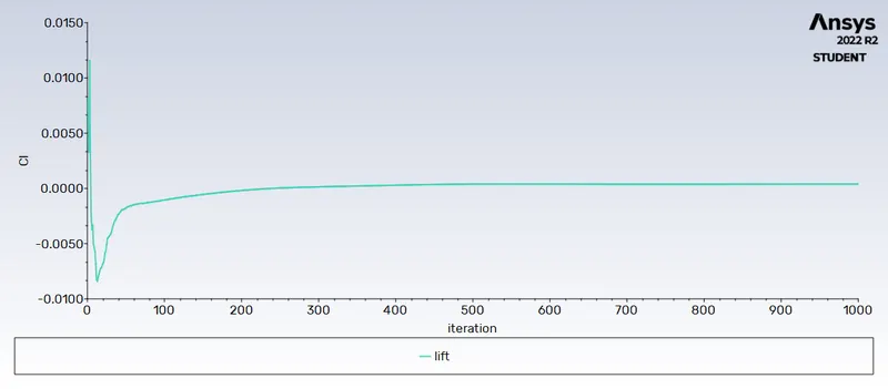
fig 17 lift coeffiecient
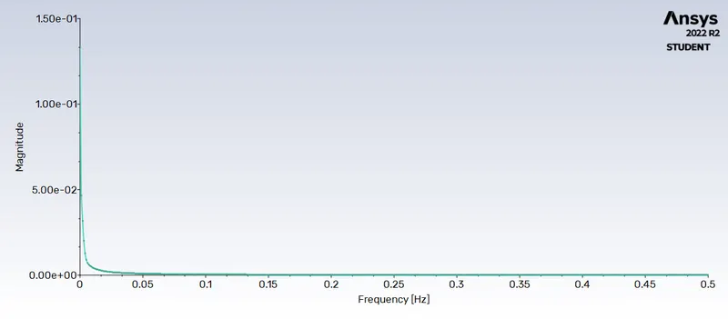
fig 18 Strouhal Number
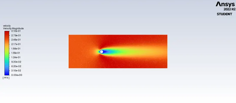
fig 20 velocity contour
Reynolds number 100
simmilarly for Re 100
v=2.5 and other parameter remains same
results of case 2 steady case Re 100
drag coeffient 13.55
lift coeffient 0.416
moniter velocity 1.35 m/s
Fig 21 residuel moniter
fig 22 moniter velocity plot
Fig 23 drag coefficent
Fig 24 Lift coefficent
fig 25 Strouhal Number
Reynolds number 1000
v=25 and other parameter remains same
results of case 2 steady case Re 1000
drag coeffient 697.47
lift coeffient 301
moniter velocity 18.523 m/s
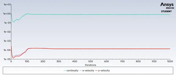
fig 26 residuel moniter
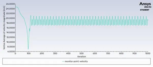
fig 27 monitor velocity
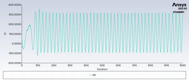
fig 28 lift coefficient
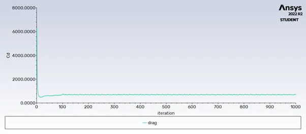
fig 28 drag coeficient
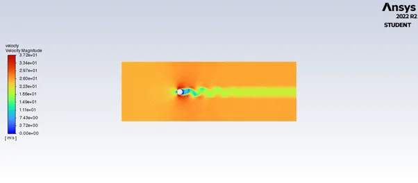
fig 30 velocity contour
Reynolds number 10000
v=250 and other parameter remains same
results of case 2 steady case Re 100
drag coeffient 78447
lift coeffient 588
moniter velocity 182.42 m/s
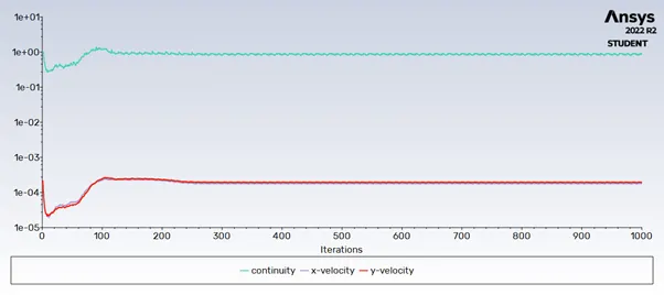
fig 31 residuel monitor
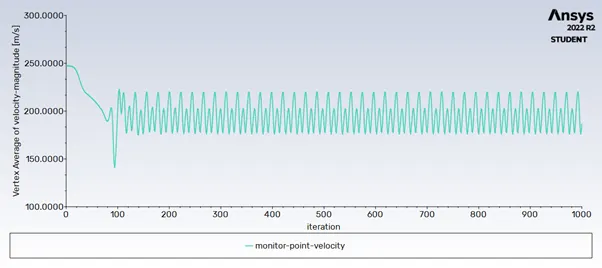
fig 32 monitor velocity
f
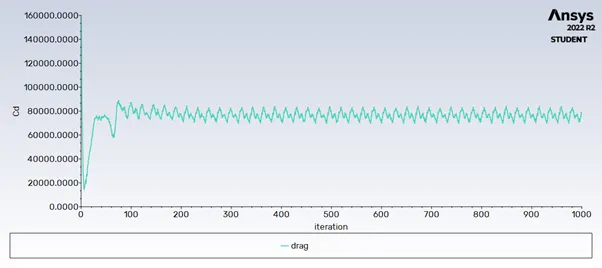
fig 33 lift coefficeint
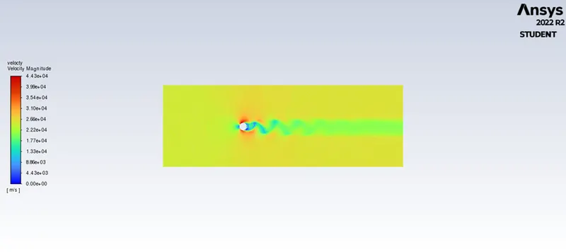
fig 34 velocity countor
Reynolds number 100000
v=25000 and other parameter remains same
results of case 2 steady case Re 100
drag coeffient 7.67*10^8
lift coeffient 3.39*10^8
moniter velocity 18537 m/s
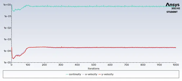
fig 35 residuel monitor
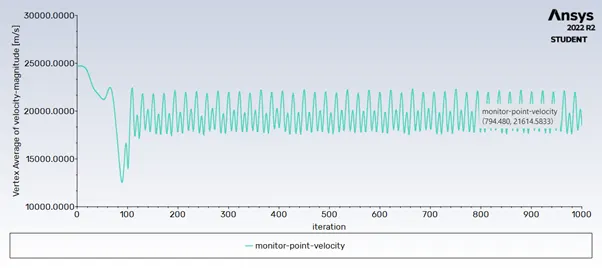
fig 36 monitor velocity
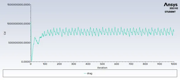
fig 37 drag coeffient
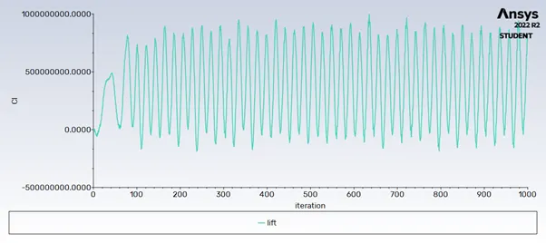
fig 38 lift coeffienent
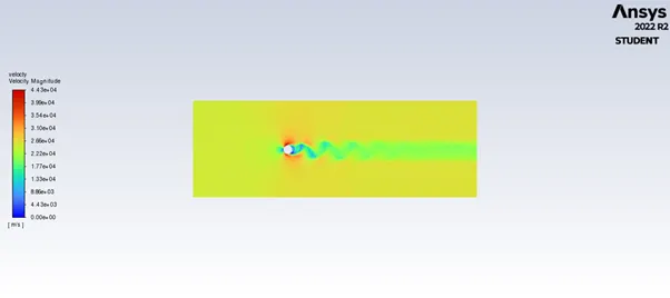
fig 39 velocity countor
results anmation s are attached to the zip file
inclusing animation
Conclusion
case 1 in both steady and unsteady case there can be seen Von karman vortex shading
case 2 except Re with 10 there is no von karman vertex is not seen other then that in every case it can be seen
in as the reynolds no increase there is increase in drag coeefient and lift coeffient