Week 2 - Flow over a Cylinder.
Aim: To simulate the flow over a cylinder and explain the phenomenon of Karman vortex street.
Objective:
- CASE-I: To Simulate the flow with the steady and unsteady case and calculate the Strouhal Number for Re= 100.
- CASE-II:
- Calculate the coefficient of drag and lift over a cylinder by setting the Reynolds number to 10,100,1000,10000 & 100000. (Run with a steady solver)
- Discuss the effect of the Reynolds number on the coefficient of drag.
FACTORS ENTAILED:
1. Flow over a cylinder:
- Flow over a cylinder is important in many industrial applications like cooling iron or cylindrical pipe
- Circular pipes have more application in heat exchangers. High-temperature flue gases flow over a circular cylinder in a cross flow.
- Depending on flow rate, fluid properties and size of the cylinder, the flow can be laminar, transition and turbulent.
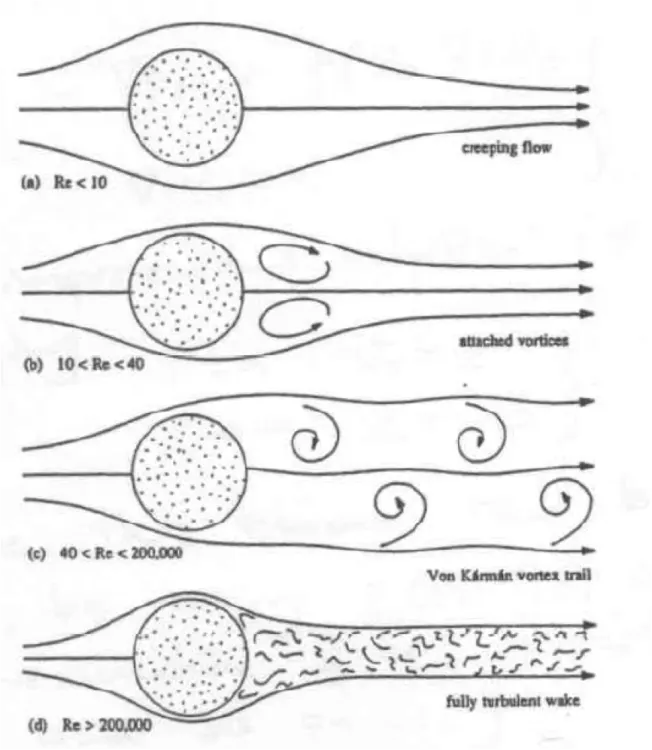
- As we can see in the picture, when Reynolds numbers<10, the flow is smooth and laminar. When Reynold's number is between 10 and 40, two stationary vortices appear behind the cylinder.
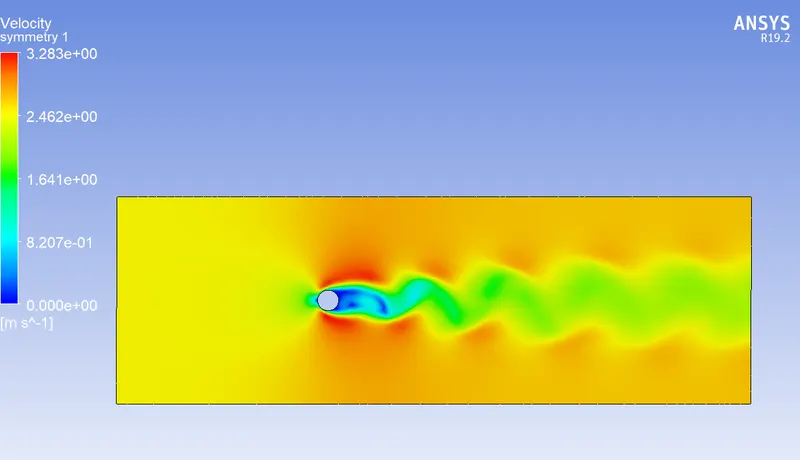
- When it is between 40 and 200, vortex shedding starts, and the vortices are going to detach from the top and bottom of the cylinder. This flow pattern is called the Von Karman Vortex Street.
2. Strouhak number:
-
It is a dimensionless number which describes oscillating flow mechanisms. It is an integral part of the fundamentals of fluid mechanics, given as
-
f is the frequency of vortex shedding, L is the diameter of the particle and V is the fluid velocity. The Strouhal Number represents the ratio of inertial forces due to the unsteadiness of the flow or local acceleration to the inertial forces due to changes in velocity from one point to another in the flow field.
Where,
f= frequency of vortex shedding
L= characteristic diameter of the cylinder
V= fluid flow velocity
3. Co-efficient of drag:
-
In fluid dynamics, the drag coefficient is a dimensionless quantity that is used to quantify the drag or resistance of an object in a fluid environment, such as air or water. It is used in the drag equation in which a lower drag coefficient indicates the object will have a less aerodynamic or hydrodynamic drag. The drag coefficient is always associated with a particular surface area.
-
The drag coefficient of any object comprises the effects of the two basic contributors to fluid dynamic drag: skin friction and form drag. The drag coefficient of a lifting airfoil or hydrofoil also includes the effects of lift-induced drag. The drag coefficient of a complete structure such as an aircraft also includes the effects of interference drag.
4. Co-efficient of lift:
-
The lift coefficient is a dimensionless coefficient that relates the lift generated by a lifting body to the fluid density around the body, the fluid velocity, and an associated reference area. A lifting body is a foil or a complete foil-bearing body such as a fixed-wing aircraft. CL is a function of the angle of the body to the flow, its Reynolds number, and its Mach number.
-
The section lift coefficient cl refers to the dynamic lift characteristics of a two-dimensional foil section, with the reference area replaced by the foil chord.
- SOLUTION:
CASE 1: (a) STEADY-STATE
PROCESS: GEOMETRY
- All the units are in meters
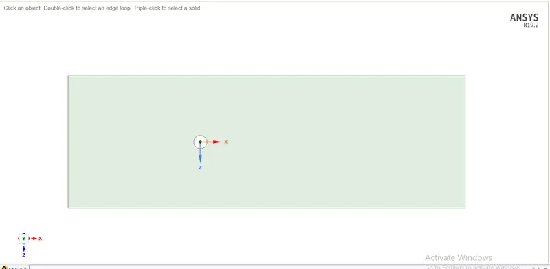
- The diameter of the circle is 2 m, the total triangle length is 60x20m, and the distance from the midpoint of the circle to the breath end is 10m.
Mesh:
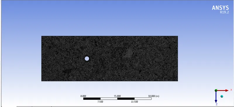
- After the geometry is loaded we should mesh it and here I used 0.25 m as elemental size.
-
But in the meshing nodes, the shape is more quadrilateral than the triangle so we should do this by changing the method to the triangle in the insert option
-
After changing the node's shape into triangles we should improve the mesh around the cylinder by sizing in the mesh which is used to control precisely the mesh.
-
Then we should add inflation which is used to create a body-fitted mesh.
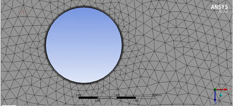
- And we should name the boundaries as given below,
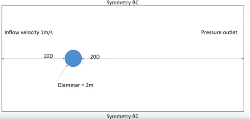
- where the cylinder edge is named as walls.
Data for Setting up Ansys fluent:
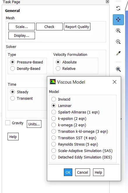
- We should update the mesh before opening the setup. Then, we should change from a viscous to a laminar flow.
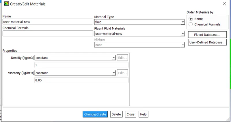
- Open Materials and enter the density and kinematic viscosity values for the fluid that will be used in the simulation in this case, air.
Reference values:
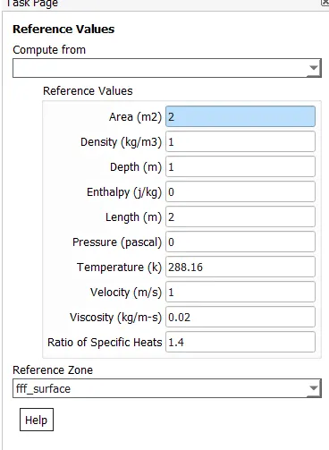
- Density/kinematic viscosity: 1/0.05
- Create a monitor point behind the cylinder by selecting the point under surfaces in the results bar.
- After creating the monitor point, create reports/plots for drag, lift, velocity wrt cylinder.
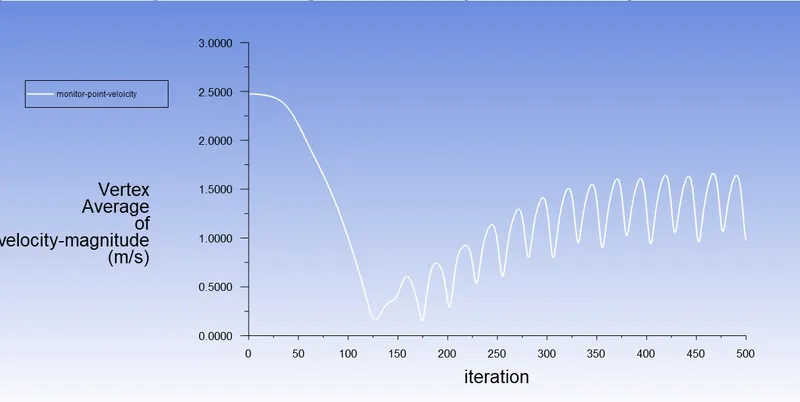
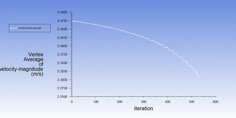
- Create plots for the velocity at the monitor point to analyze the vortex shedding. Use hybrid initialization for steady-state and standard for transient state simulations.
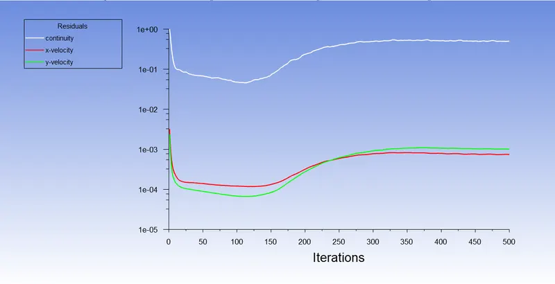
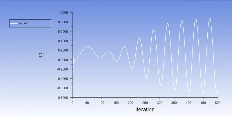
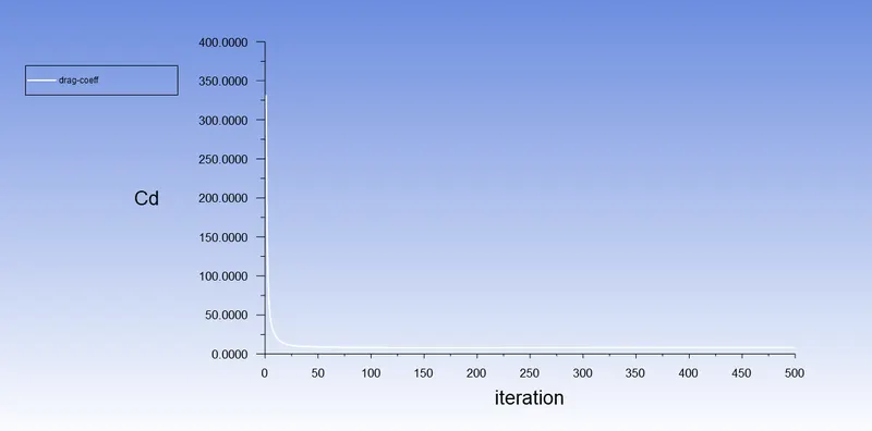
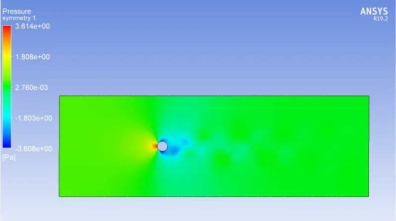
NOW, Simulate the flow with the steady case and calculate the Strouhal number for Re=100 and velocity 2.5m/s.
- Residuals plot:
- Monitor point velocity:
- Coefficient of lift (Cl):
- Coefficient of drag (Cd):
- Pressure contour:
- Velocity contour:
CASE 1: (b) UN-STEADY STATE:
NOW, Simulate the flow with the unsteady case and calculate the Strouhal number for Re=100 and velocity 2.5m/s.
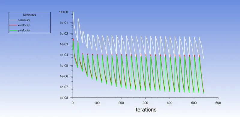
- Residuals plot:
- Monitor point velocity:
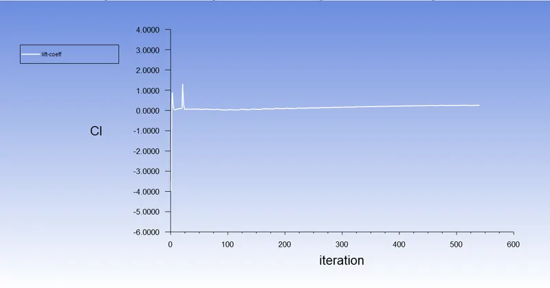
- Coefficient of lift (Cl):
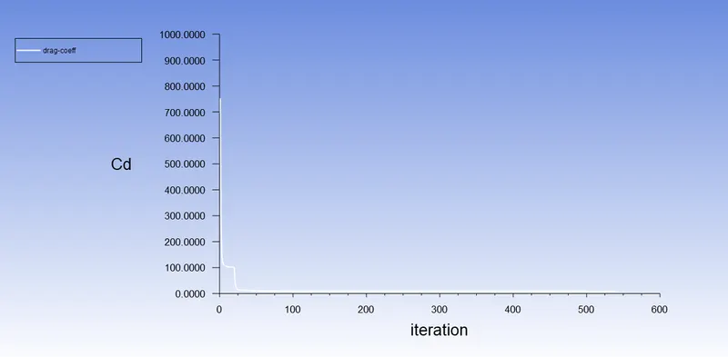
- Coefficient of drag (Cd):
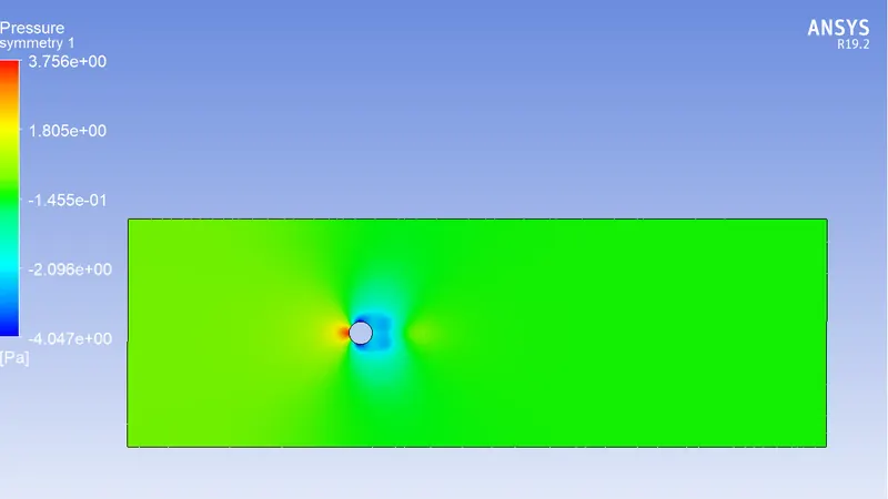
- Pressure contour:
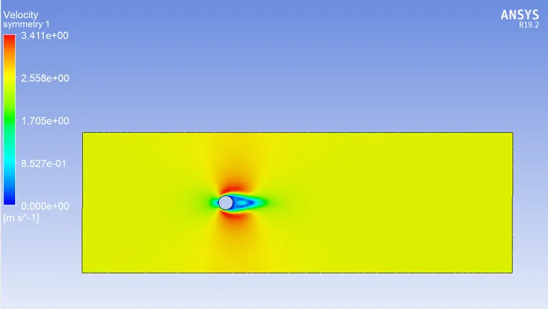
- Velocity contour:
CASE 2:
(1) STEADY-STATE :
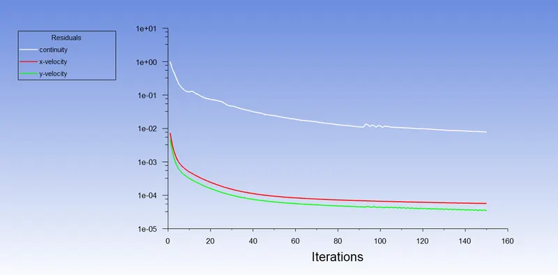
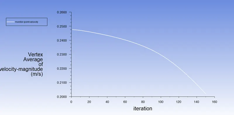
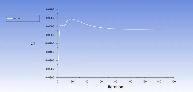
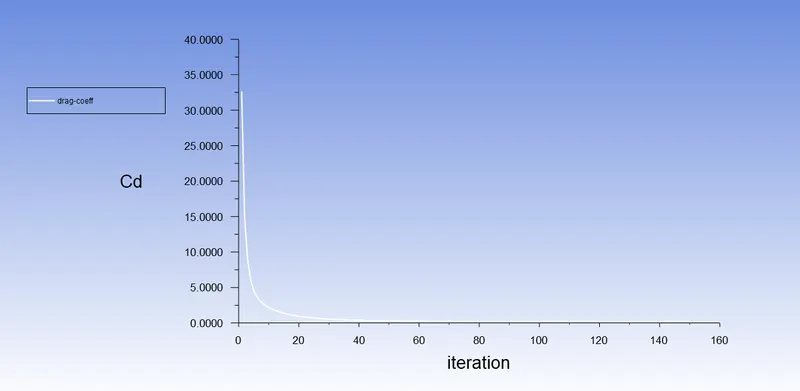
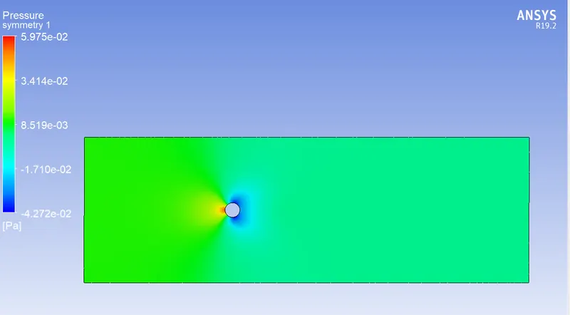
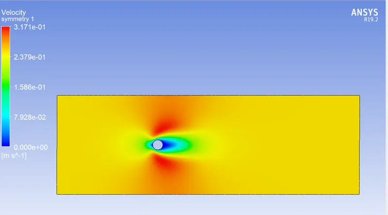
NOW, Simulate the flow with the steady-state solver for Re=10.
Where,
Re=10, velocity v=0.25m/s
- Residuals plot:
- Monitor point velocity:
- Coefficient of lift (Cl):
- Coefficient of drag (Cd):
- Pressure contour:
- Velocity contour:
(2) STEADY-STATE :
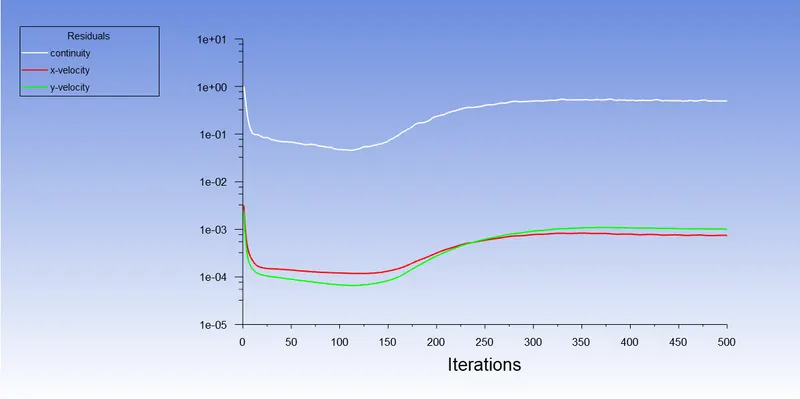
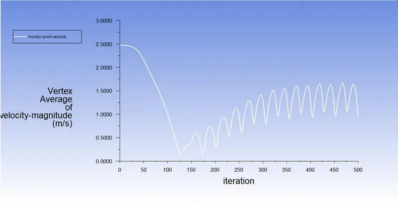
NOW, Simulate the flow with the steady-state solver for Re=100.
Where,
Re=100, velocity v=2.5m/s
- Residuals plot:
- Monitor point velocity:
- Coefficient of lift (Cl):
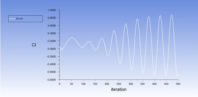
- Coefficient of drag (Cd):
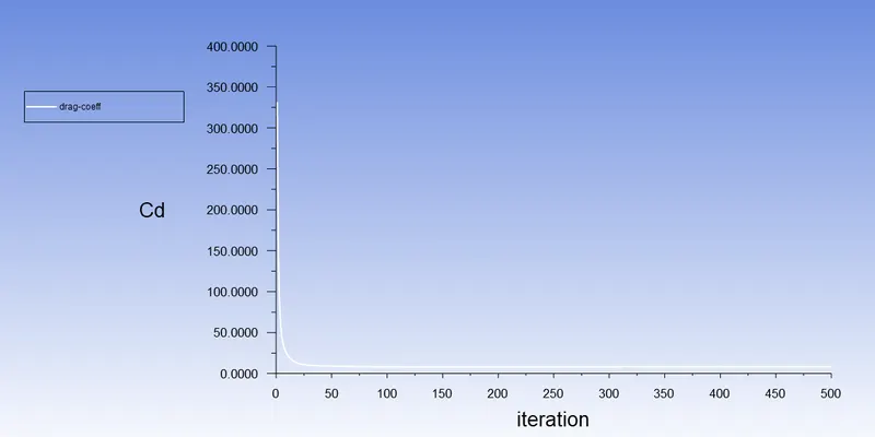
- Pressure contour:
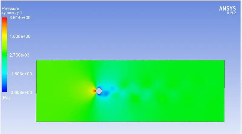
- Velocity contour:
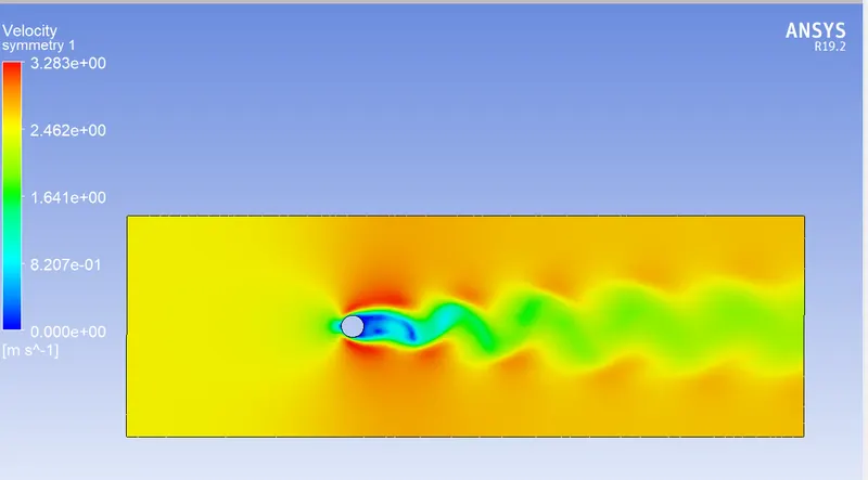
(3) STEADY-STATE :
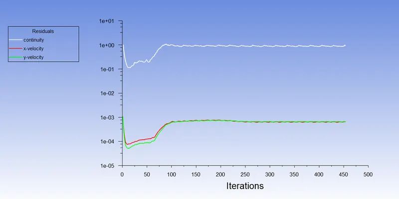
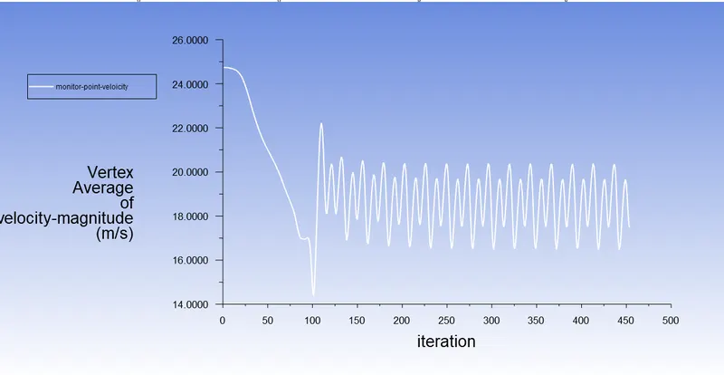
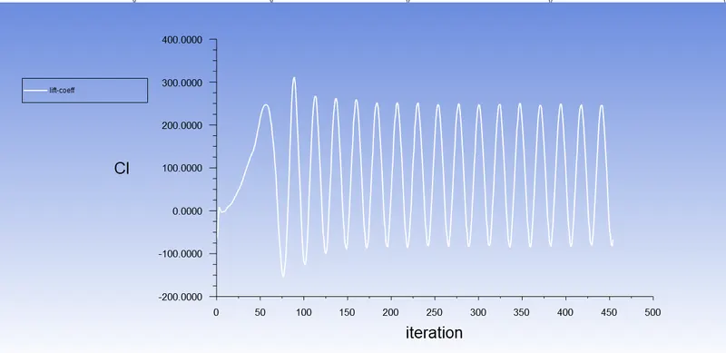
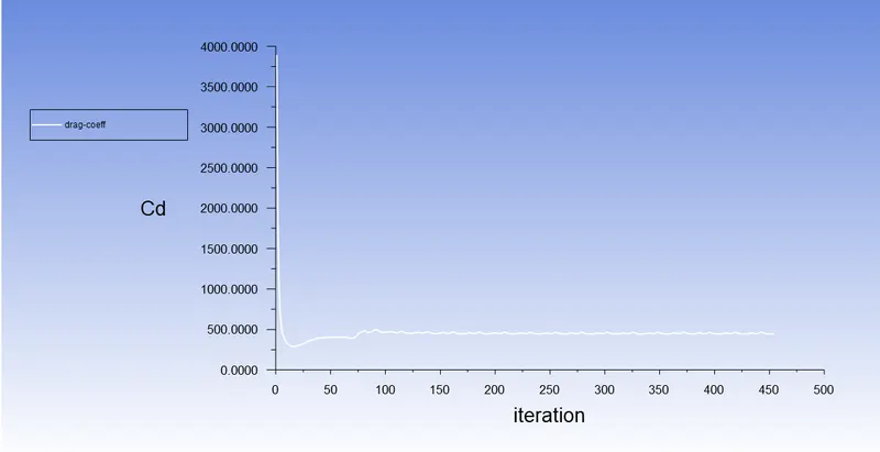
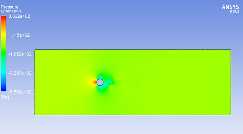
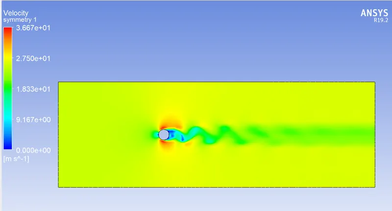
NOW, Simulate the flow with the steady-state solver for Re=1000.
Where,
Re=1000, velocity v=25m/s
- Residuals plot:
- Monitor point velocity:
- Coefficient of lift (Cl):
- Coefficient of drag (Cd):
- Pressure contour:
- Velocity contour:
(4) STEADY-STATE :
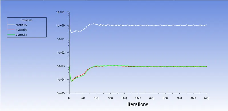
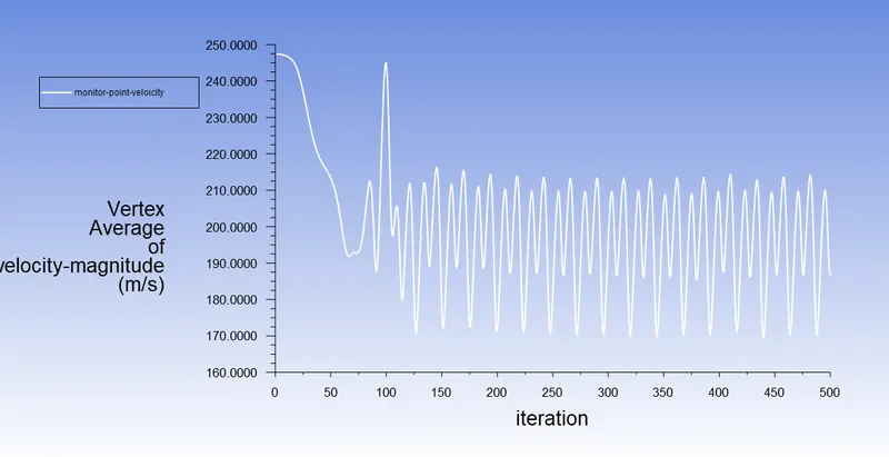
NOW, Simulate the flow with the steady-state solver for Re=10000.
Where,
Re=10000, velocity v=250m/s
- Residuals plot:
- Monitor point velocity:
- Coefficient of lift (Cl):
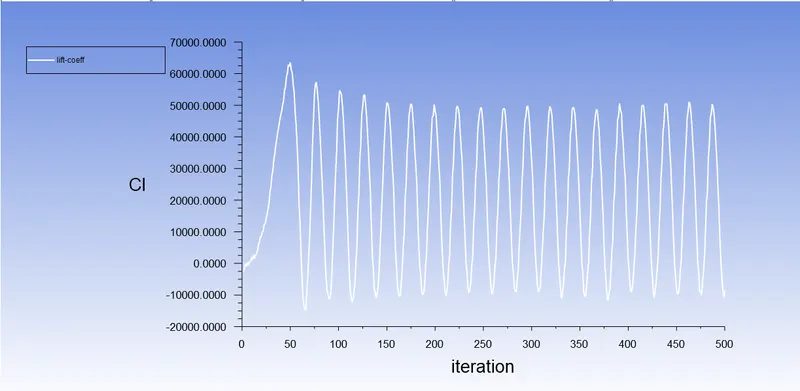
- Coefficient of drag (Cd):
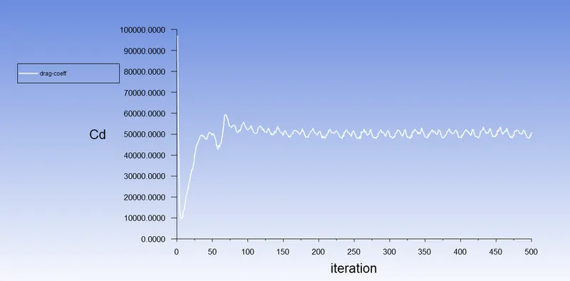
- Pressure contour:
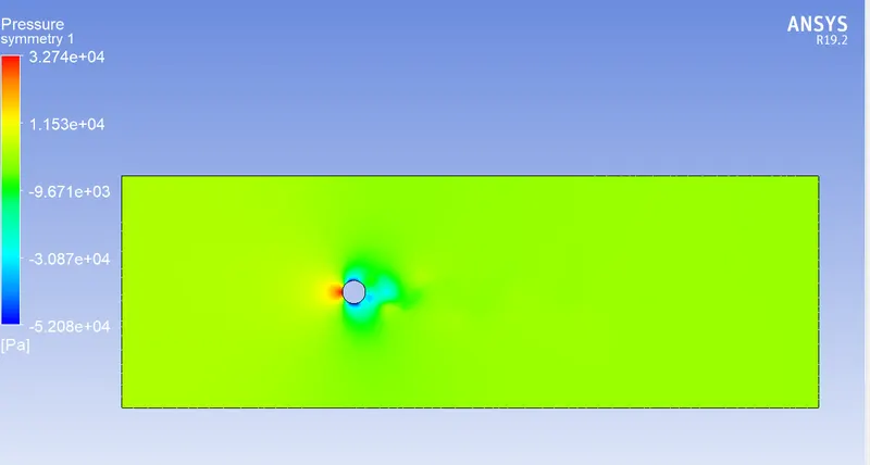
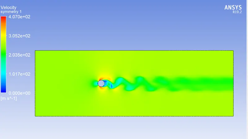
- Velocity contour:
(5) STEADY-STATE :
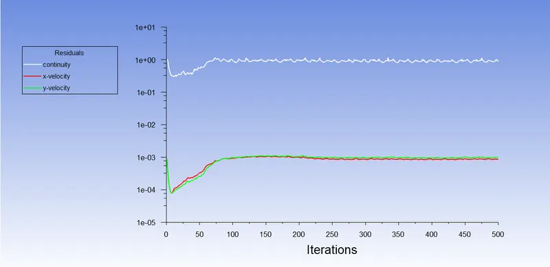
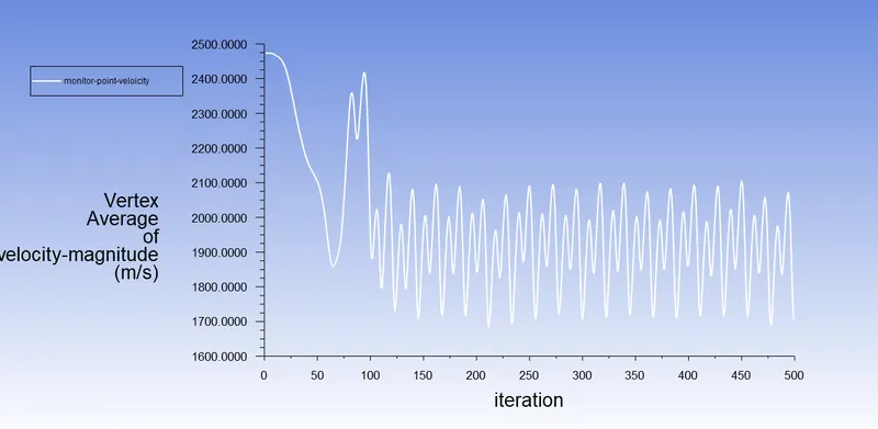
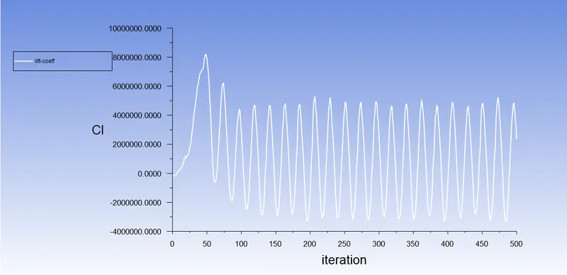
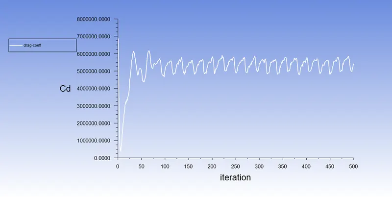
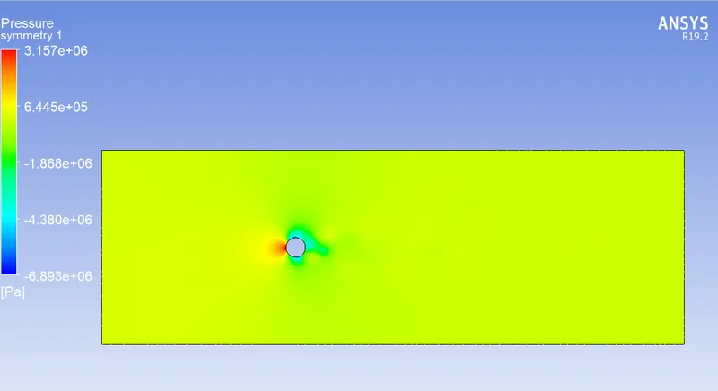
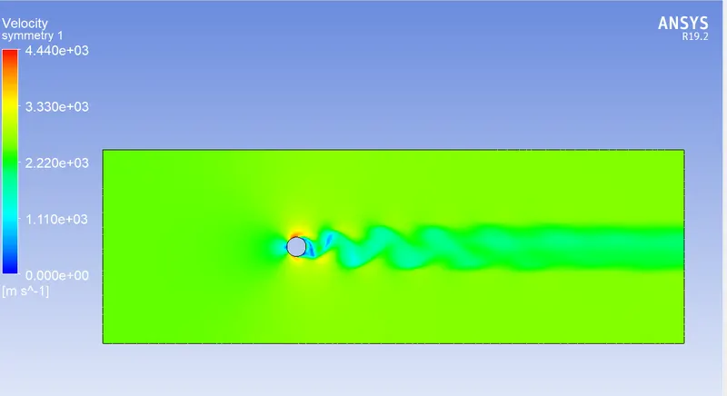
NOW, Simulate the flow with the steady-state solver for Re=100000.
Where,
Re=100000, velocity v=2500m/s
- Residuals plot:
- Monitor point velocity:
- Coefficient of lift (Cl):
- Coefficient of drag (Cd):
- Pressure contour:
- Velocity contour:
RESULT:
Drag and lift coefficient for different Re:
`R_e` `C_d` `C_l`
10 3.45 -0.01
100 1.13 -0.120
1000 0.98 -0.050
10000 0.95 -0.035
100000 0.87 -0.023
Errors with respect to the theoretical values from the reference material,
| Reynolds number | Theoretical Cd | Numerical Cd | error |
| 10 | 3.5 | 3.154 | 4.54% |
| 100 | 1.4 | 1.857 | 3.2% |
CONCLUSION:
- The flow over a cylinder is simulated in the first case for both steady and unsteady cases with Re=100, and from the results, the Von Karman Vortex Street phenomenon is also seen.
- Plots that are necessary to see that the flow has converged and that vortex shedding is occurring are created. Hence, to observe the flow over a cylinder, contours are created.
- In the second instance, The Reynolds number is changed in six different simulations, i.e. (Re = 10,100,1000,10000,100000,1000000), to observe how the drag and lift coefficients behave. The Reynolds number is changed by varying the flow velocity while holding the other parameters constant in order to observe how the drag coefficients behave in the simulations.
- For Re=10, it is observed that there is no formation of vortex shedding and in the rest of the cases, it is clearly observed.
- At a higher Reynolds number, flow around the cylinder becomes irregular. The increased inertia forces break the vortex generated behind the cylinder, with a higher frequency of vortex shedding than that in laminar flow
- From the above table, it can be concluded that the error percentage is less than 5%.
REFERENCE: