Week 2 - Flow over a Cylinder.

Aim : - Vortex shedding simulation over a cylinder in Laminar flow.

Introduction: - Flow over a cylinder is one of the basic simulation in the CFD domain and till this date the research is still going on to study the unsteady behaviour caused by the flow. The flow over cylinder is study is very complex and periodic flow pattern are seen at lower Reynolds number and after achieving critical Reynolds number value, the flow gets change in the wake region and the wake formation can be studied using literature of Von karman vortex street. consider any other object compared to cylinder most of them cause boundary layer detachment due to the effect of geometry like sharp edges but in the case of cylinder the point of seperation is very complex and depend upon nature of upstream boundary layer and other flow parameters.

Laminar region to turbulent region is govern by the dimensionless number called Reynolds

Vortex shedding is an oscillating flow that takes place when a fluid such as air or water flows past a bluff (as opposite to streamlined) body at certain velocities, depending on the size and shape of the body. In this flow vortex are created at the back of the body and detach periodically from either side of the body forming a Von Korman vortex street

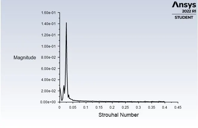
Strouhal number :

In dimensional analysis, the strouhal number is a dimensionless number describing oscillating flow mechanisms.

For large strouhal number (order of 1), viscosity dominates flow fluid, resulting in a collective oscillating movement of the fluid "plug'. For low strouhal numbers(order of 10^-4 and below ), the high speed,quasi-steady-state portion of the movement dominates the oscillation .Oscillation at intermediate strouhal numbers is characterized by the buildup and rapidly subsequent shedding of vortices.

The strouhal number is often given as

`S_t = fD`\`S_t = {fD}/{U'}`

where

f = frequency of vortex shedding

D = characteristic diameter of the cylinder]

U' = fluid flow velocity

Solving and Modelling Approach:-

The main aim of the project isto study the behavior of Reynolds number on the flow over cylinder. To capture the flow with every regime it is important to have more flow domain and less mesh size to capture every possible vortex in wake region.

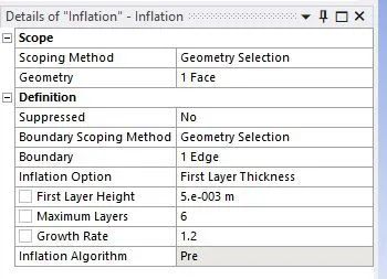
The problem is divided into two group in which both steady and unsteady state simulation will be carried accordingly. In steady state simulation the varying Reynolds number will be taken into consideration by maintaining fluid property constant. The simulation will be running for 10,100,1000,10000,100000 Reynolds number and accordingly other parameters will be studied. The problem will start with 2D geometry of flow field and mesh afterward. It is important to have less mesh size to capture every little details from flow domain. The inflation layer will be added near the cylinder to capture boundary layer detachement from the surface of cylinder. As it is stand to perform the unsteady state simulation this project will incorporate special method to solve the problem with traditional method and NITA method. i.e non iterative time advancement. This solver is more toward solving time marching problem with greater ease and with less number of iteration. The boundary conditions wil be simple as velocity inlet and pressure oulet with symmetry wall type condition. The cylinder will be also considering as wall type on which coefficientof lift and drag will be calculated

Procedure :

Geometry :

For modelling the approach we are starting with the creation of geometry. first we get into the geometry section where we create the geometry using the Space claim.

A plate with the dimension of 20*60m is created using Spaceclaim.

First we select the unit in meters are required dimensions are given we create the geometry using the tools.

We remove the extra edges using the deleting construction lines.

We use pull command to make it a surface.

We remove the circular area to create the cylinder.

Procedure :

Geometry :

For modelling the approach we are starting with the creation of geometry. first we get into the geometry section where we create the geometry using the Space claim.

A plate with the dimension of 20*60m is created using Spaceclaim.

First we select the unit in meters are required dimensions are given we create the geometry using the tools.

We remove the extra edges using the deleting construction lines.

We use pull command to make it a surface.

We remove the circular area to create the cylinder.

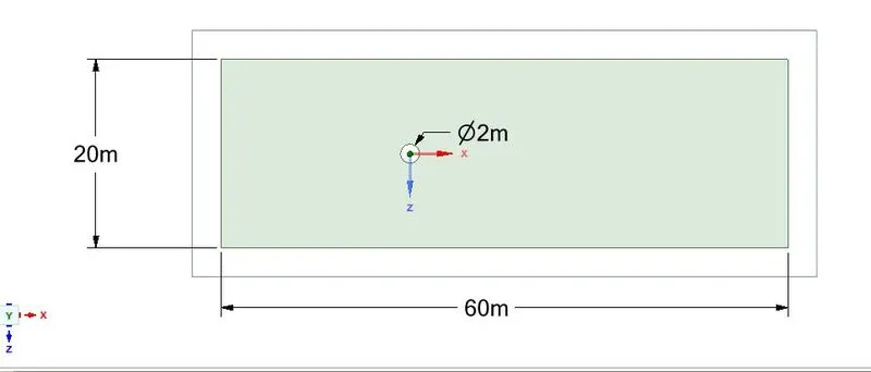
Now, we want to simulate effect of fluid flow over cylinder, select the circle and delete it.

Meshing :

We use a meshing tool to mesh the geometry.

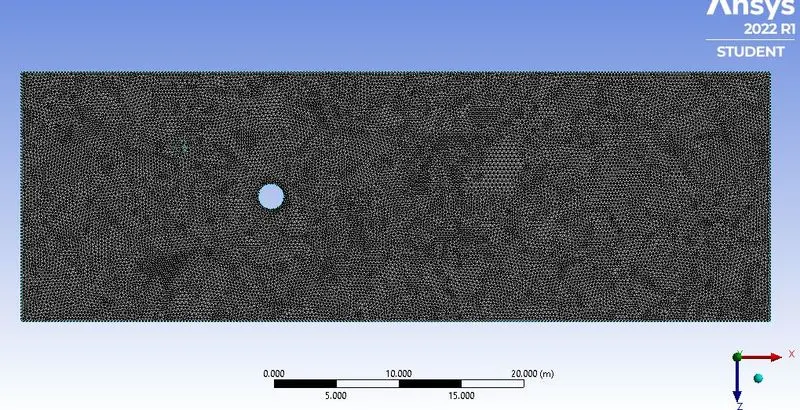
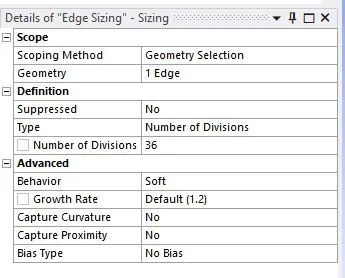
First we create the mesh by giving the element size i.e 0.25 meters.

To make sure that FLUENT read the boundary conditions from workbench named selection should be provided according to flow parameters. The problems has velocity inlet and pressure outlet boundary conditions. The cylinder is considering as well as other two edges are considering as symmetry boundary conditions.

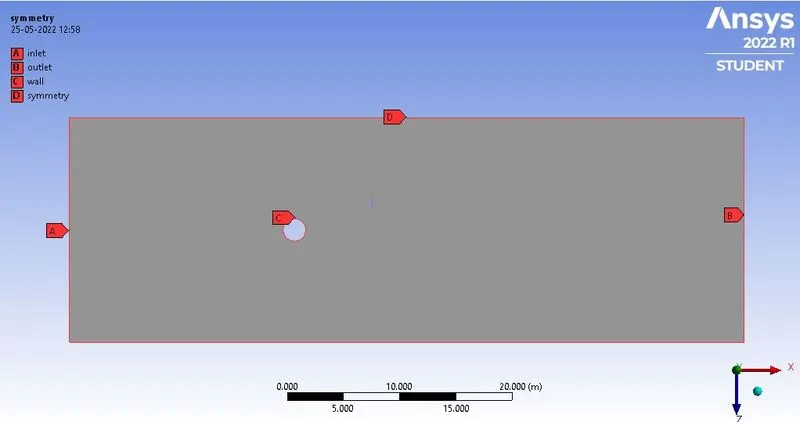
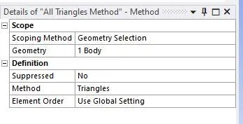
and we convert the quad dominated mesh into traingle dominated mesh.

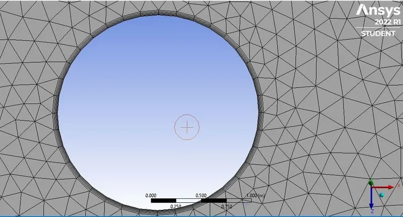
we have to capture the physics at the circumference of the cylinder is perfectly so we divide circle into 6 parts.

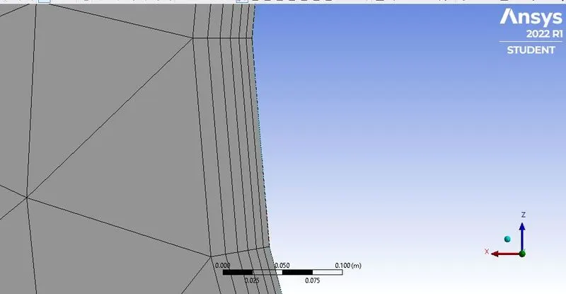
and then to create body fitted mesh we are adding the inflation layers to capture the physics more clearly.

if we are not getting the correct results for the results size, again we change the mesh size to capture solution correctly.

after meshing we create the named selection of boundary.

we gave the name to each of the faces of the boundaries.

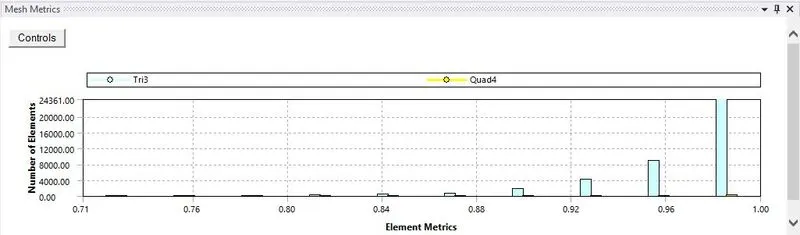
The mesh quality which need to checked are skewness and orthogonal quality of elements. The skewness quality should have most element near to 0 which show better element quality and opposite to skewness , orthogonal quality should have more element near to 1 which represents better quality of elements.

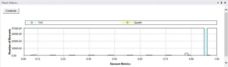
Orthogonal quality

Setup :

we are using the pressure based solver because the mach number is less then 0.8

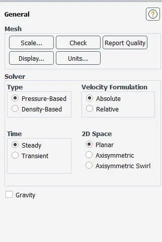
and steady state because are not solving the time derivative.

we only solve time derivative when we want time-accurate solution. how many quantities are changing according to the time.

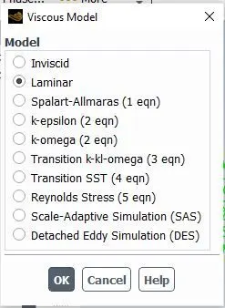
we are using the viscous laminar model because flow is laminar.

we create the user defined material which has viscosity of 0.05m^2/s and density of air is 1kg/m^3 because we have to see how vortex shedding is happening.

then we apply the required boundary condition as the problem.

Open material and create a fluid that is to be used for simulation for this case, it is air and also inputs the density and kinematic viscosity values.

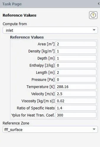
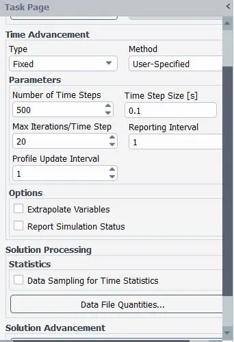
Open zones and input the inlet velocity as per the reynolds number and check if the fluid is updated

Update the references values which is located inside set up at the right-hand side.

GRID INDEPENDENCE TEST :

Grid independence is the test where we took the results for different sizes of mesh. and we select the optium meesh means course mesh than other which gave us the same results. In other words the further decreases in the element size does not effect the solution because the error is very small.

We choose the mesh which gave us the same result, but has a bigger element size to reduce the computational time.

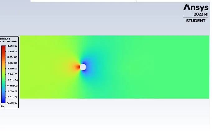
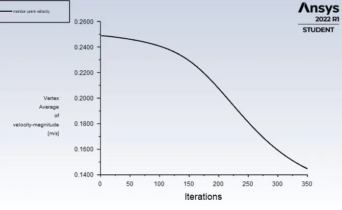
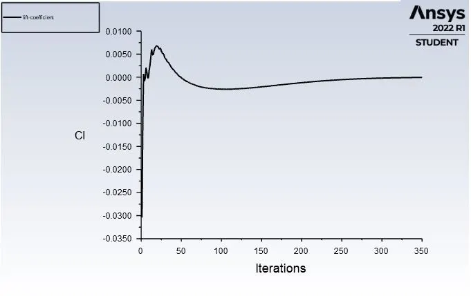
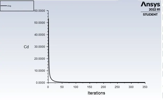
RESULTS FOR THE REYNOLDS NUMBER 10

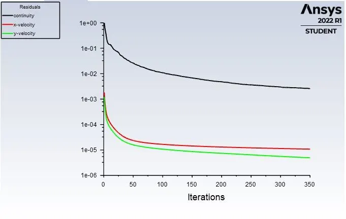
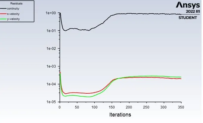
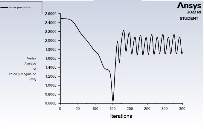
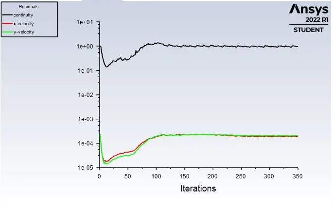
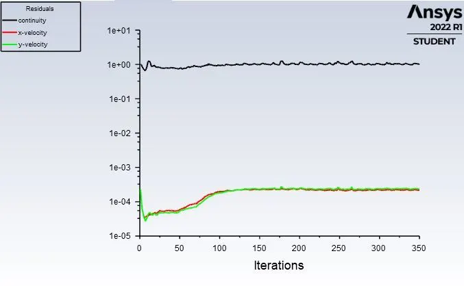
After initialization of solution we run the simulation for 350 iteration. Here convergence is not manily important parameter to consider rather than that flow has to be stabilize for longer period so as to capture vortices in the wake region of flow domain.

• Residual Plot

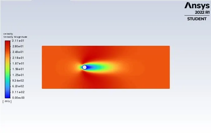
• Velocity and pressure contours

• Velocity at the monitor point

• Lift and Drag Coefficient

RESULTS FOR THE REYNOLDS NUMBER 100

• Residual plot

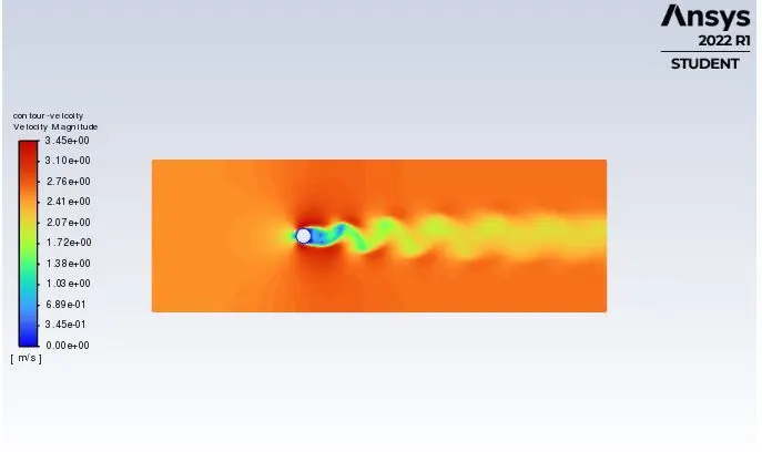
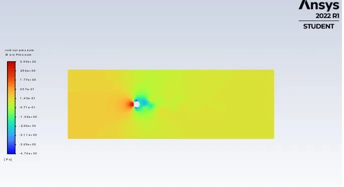
• Velocity and Pressure contours

• Velocity at the monitor point

• Drag and lift coefficient

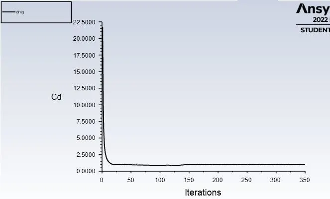
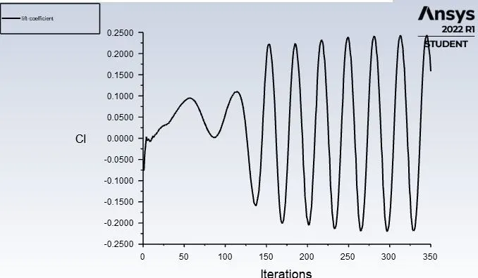
Strouhal number plot

RESULTS FOR THE REYNOLDS NUMBER 1000

• Residual plot

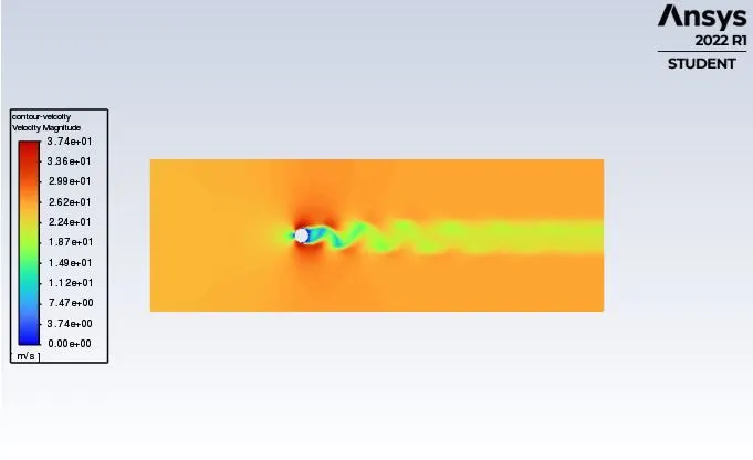
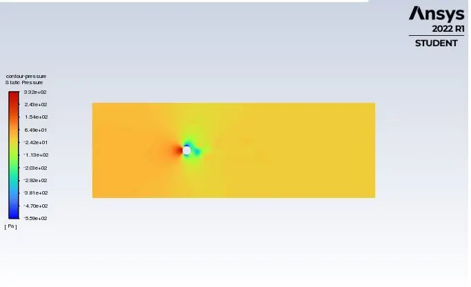
• Velocity and pressure contours

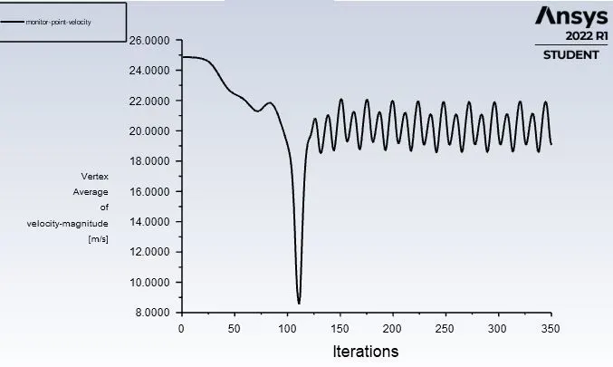
• Velocity at the monitor point

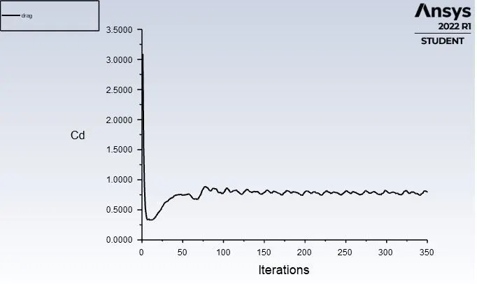
• Drag and lift coefficient

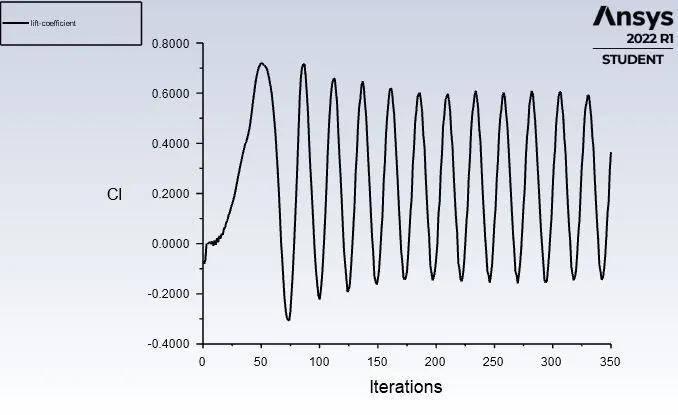
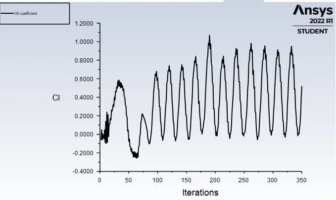
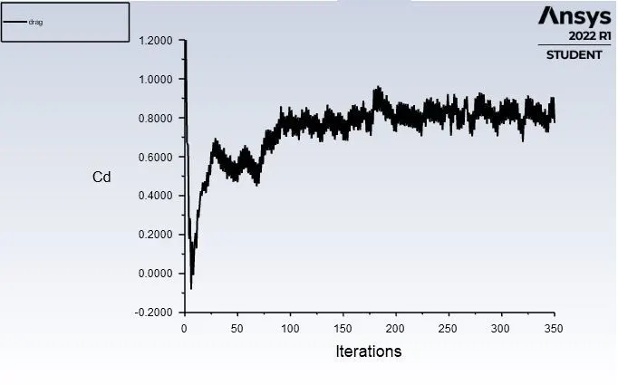
RESULTS FOR THE REYNOLDS NUMBER 10000

• Velocity and pressure contours

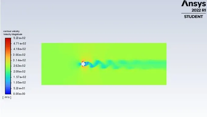
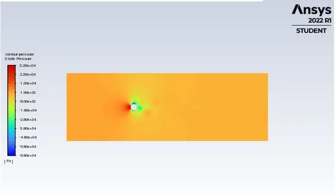
• Residual plot

• Velocity at the monitor point

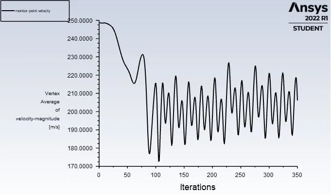
• Lift and drag coefficient

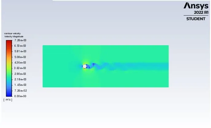
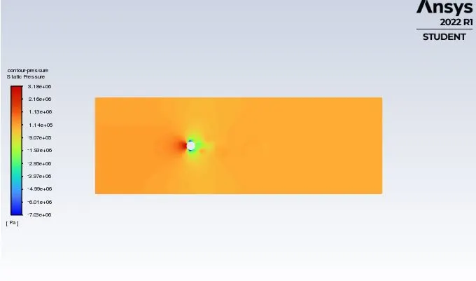
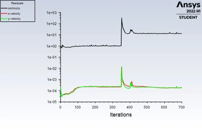
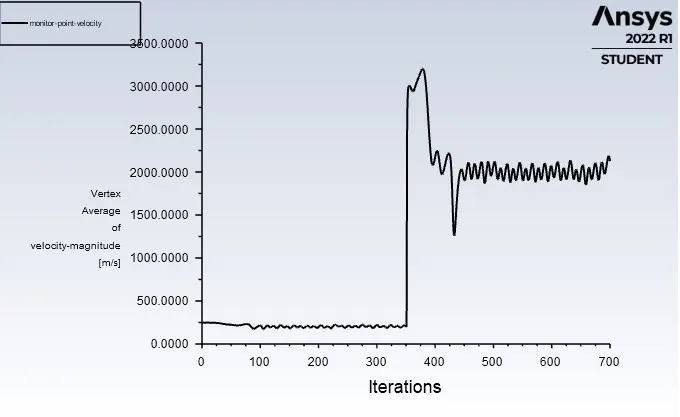
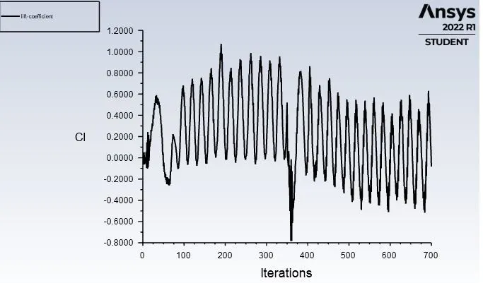
RESULTS FOR THE REYNOLDS NUMBER 100000

• Velocity and pressure contours

• Residual plot

• Velocity at the monitor point

• Lift and drag coefficient

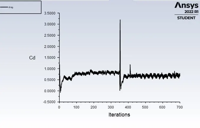
RESULTS FOR THE REYNOLDS NUMBER 100 FOR TRANSIENT STATE

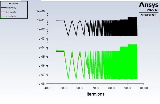
In the Transient state for Re = 10, here i gave values of Number of Time steps is 100 and time step size 0.1s and i am going to give Run calculation figure given below -

Residual plot

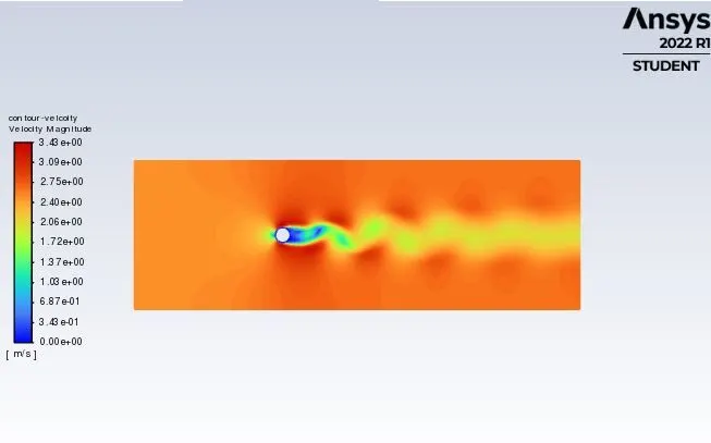
Pressure and Velocity contour

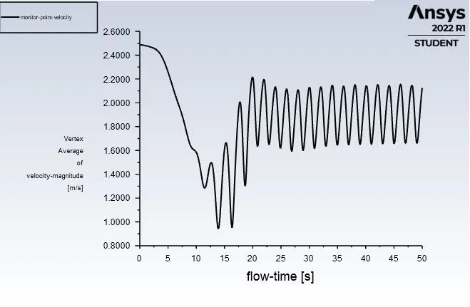
Monitor-point-velocity

Drag and Lift co-efficient

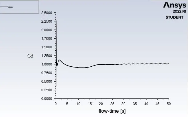
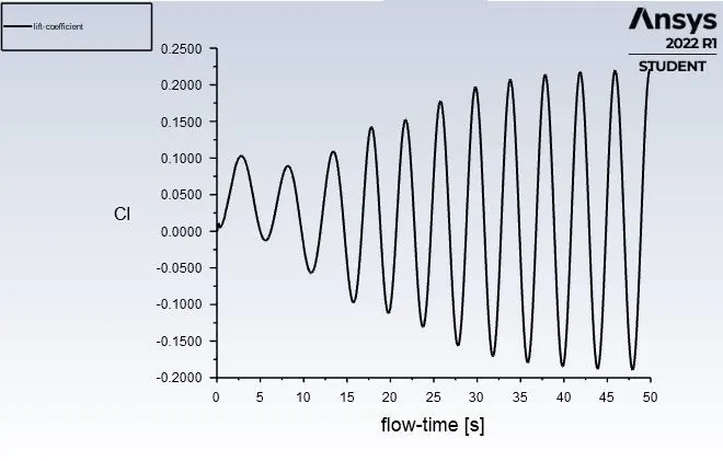
Strouhal number plot

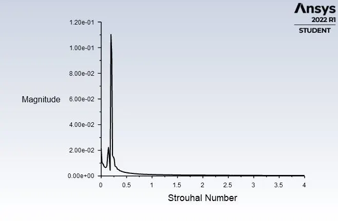
Results : -

Drag and lift coefficient for different Re

State of fluid	Reynolds number (Re)	Co-efficient of drag (`C_d`)	Lift Co-efficient (`C_l`)
Steady	10	2.12604	0.006125
Steady	100	1.0439	0.158191
Unsteady	100	1.0172531	0.21961093
Steady	1000	0.79263	0.364847
Steady	10000	0.77325	0.52069
Steady	100000	0.662155	-0.0827128

Conclusion :-

• In the first case, the flow over a cylinder is simulated for both steady and unsteady cases with Re = 100, and with the results generated the phenomena of Von Karman Vortex Street is also observed.
• Necessary plots are plotted in order to observe that the flow is converged and the vortex shedding is happening.
• Contours are generated in order to observe the flow over a cylinder.

• In the second case,
• Six different simulation i.e ( Re = 10,100,1000,10000,100000) are simulated to observe the behaviour of drag and lift coefficient by changing the Reynolds number.
• In order to observe the behaviour of the drag coefficients for the simulations , the velocity of the flow is varied to change the Reynolds number and the rest of the parameters are kept constant.
• As we know that if the Reynolds number is less than 2000, the flow in a pipe is Laminar. Hence we use the Viscous model = Laminar.
• For Re = 10, it is observed that there is no formation of Vortex shedding and in the rest of the cases, it is clearly observed.
• As per the basic conditions and parameters, the results are validated from the literature.
• As we refine the mesh we need to run more iterations, that's basically a common sense.
• From the above table values, it can be concluded that the error percentage is less than 5%

Reference Article

https://www.sciencedirect.com/science/article/pii/S0307904X08000243

Make animation video :

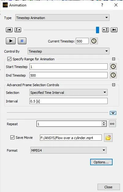
First of all , In Anys fluent after run the simulation click on playback icon and save this to the directory.

Next, In the postprocessing click on the video icon button and there one of the pop up window is coming out as a timesetep Animation and play the animation and then click on save icon and chpoose the location to save the animation file .

Youtube Animation video link

https://youtu.be/bZiT1mOkgak