Week 2 - Flow over a Cylinder.
AIM:
The objective of the report is to simulate flow over a cylinder and explain the phenomenon of Karman vortex street. The flow should be simulated for various Reynolds number using transient and steady-state solvers and results such as Strouhal number, coefficient of lift and coefficient of drag should be validated.
THEORY:
Vortex flow -
In fluids, vortex flow means the fluid is in circular motion rotating about a center point. It is a rotary flow about an axis and has no radial component of velocity.
For the uniform flow of fluid, vortices are produced only at the boundaries.
They are caused by -
- Tangential acceleration at boundaries.
- Tangential pressure gradients acting along the boundaries.
The vortex flow is created by shear flow. It has low pressure at its center.
Vortex Shedding -
In fluid dynamics, Karman vortex street is a repeating pattern of swirling vortices caused by a process known as vortex shedding formed due flow around blunt bodies.
Any obstacle present in the fluid flow, due to adverse pressure gradient, the flow gets seperated at the boundary of the obstacle. The interaction of the two seperated boundary layers causes vortex shedding. The interaction of two separated shear layers causes unsteadiness in the flow leads to flow-induced vibrations.
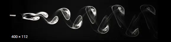
Fig - Vortex shedding due to flow of air around circular cylinder
The alternative formation of Vortex on top and on bottom of the cylinder and passing of the vortex is called as shedding.
When, the magnitude of the frequency induced due to vortex shedding is same as natural frequency of obstacle/blunt body, resonance phenomena ocuurs which leads to catastrophic failure of the structure. So, it is important monitor and control the vortex shedding frequency.
Strouhal number -
Strouhal number is a non-dimensional number that is used to describe the frequency of the oscillating flow.
St = f*D/u , where f - frequency of vortex shedding
D - Chracteristic length of obstacle
u - free stream velocity
PROCEDURE:
In this report, simulation of flow over a cylinder is done for different Reynolds numbers like - 10,100,1000,10000,100000.
Case 1(a) - Simulation of flow for Re = 100 - transient solver
Step1 - Create the geometry in space claim
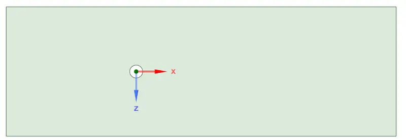
Geometric dimensions -
Cylinder diameter - 2m
Length from inlet to center of cylinder - 20m
Length from center of cylinder to outlet - 40m
Total width of domain - 20m
Step2 - Mesh generation
Boundary names should be assigned as follows
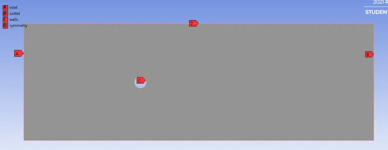
Generate triangular mesh elements of element size 0.5m
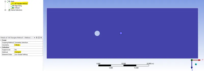
To capture the shape of the circle and to have accurate results, even no.of edges should be present on the perimeter of the circle. From experimental analysis, 36 edges on the perimeter of circle is preferred.
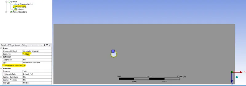
To capture the results on the boundaries accurately, finner mesh should be generated on the boundaries.
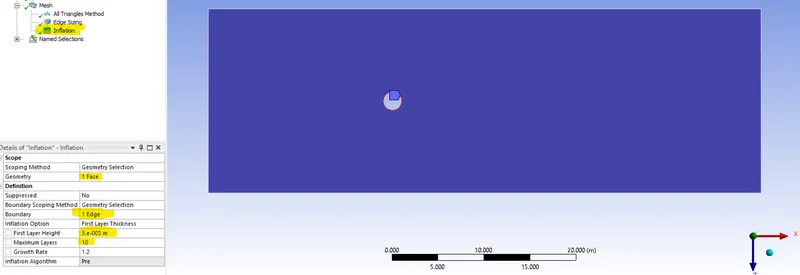
Generated mesh
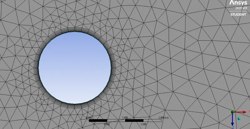
Total number of elements generated are 10,712

Step3 - Setup
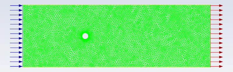
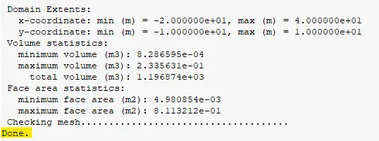
Perform mesh check. The generated mesh is of good quality
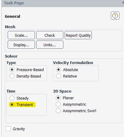
For incompressible fluids, pressure-based solver gives accurate results. Transient simulation is performed.
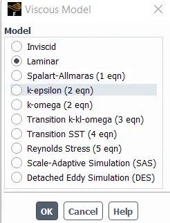
Viscous model is selected
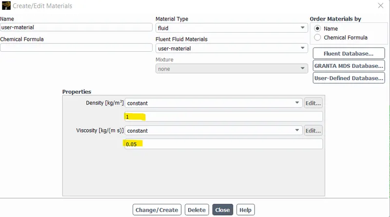
working fluid - 1) Density - 1kg/m3
2) Viscosity - 0.05 Pa-sec
Boundary-Conditions -
1) Inlet : Type - Velocity inlet
Magnitude - 2.5 m/s
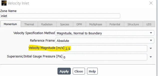
2) Outlet : Type - Pressure outlet
Magnitude - Zero gauge pressure
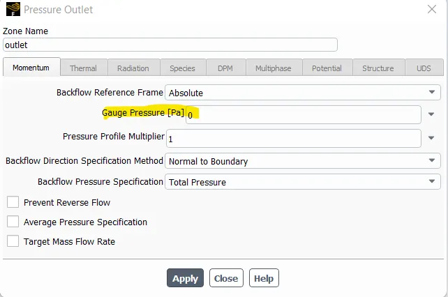
3) Walls : Type - walls
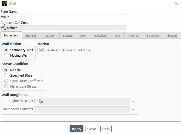
4) Symmetry : Type - Symmetry
Report plots -
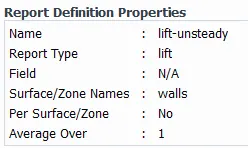
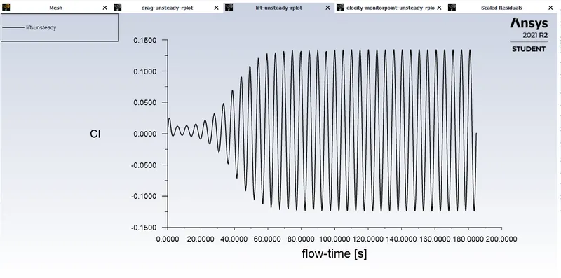
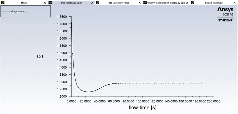
Due to vortex shedding, fluctuation of lift force acts on the obstacle. So, the aerodynamic forces like lift and drag forces need to be plotted on the wall surfaces.
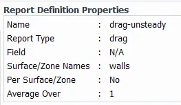
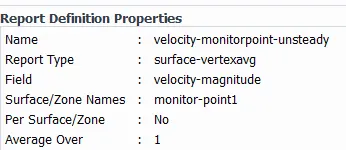
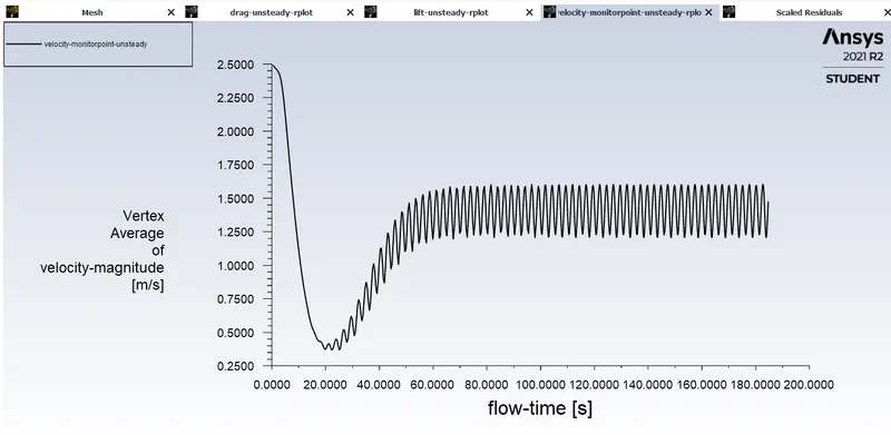
Vertex average of velocity at point (10,0) is plotted
Simulation -
Time step size - 0.1 sec
Total time - 185 sec
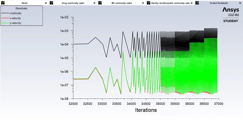
The residuals are less than 1e-3
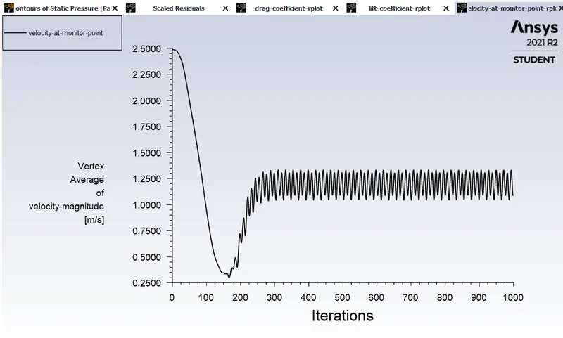
After flow time 80sec, steady-state oscillations in the velocity is obtained, which indicates convergence is achieved.
Rms value of lift coefficient is 0.091
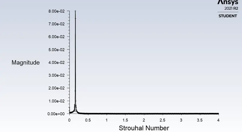
The Strouhal number is calculated at the curve peak. Strouhal number - 0.1558
Mean value of drag coefficient is 1.29
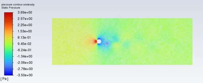
Pressure - contour
In the wake region just behind the cylinder, negative pressure is generated which is responsible for force fluctuations. The minimum pressure is of value -3.5 Pa
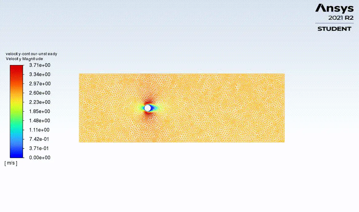
Visualization of vortex shedding
Results -
The following table shows the results for Re- 100 obtained by using transient solver.
| S.No | Strouhal number | Drag coefficient - mean value | Lift coefficient - rms value | |
| 1 | Reference value | 0.1569 | 1.3353 | 0.1792 |
| 2 | Computed value | 0.1558 | 1.29 | 0.091 |
| 3 | Absolute % error | 0.7 % | 3.39 % | 49.2 % |
Case 1(b) - Simulation of flow for Re = 100 - Steady state solver
In steady-state solver type of simulation, solver is time independent.
The input parameters and steps followed in steady-state simulation is same as transient type.
Simulation -
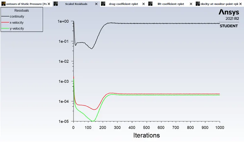
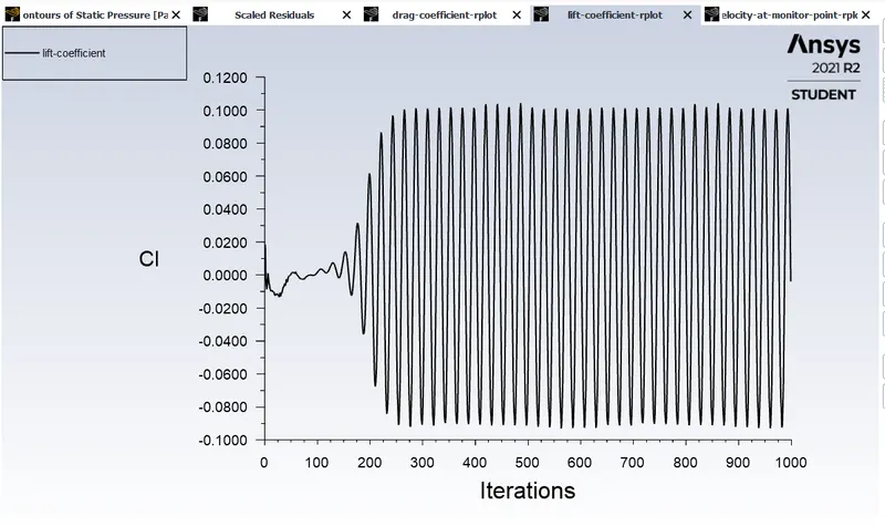
After 300 iterations, steady-state oscillations in the velocity is obtained, which indicates solution is converged.
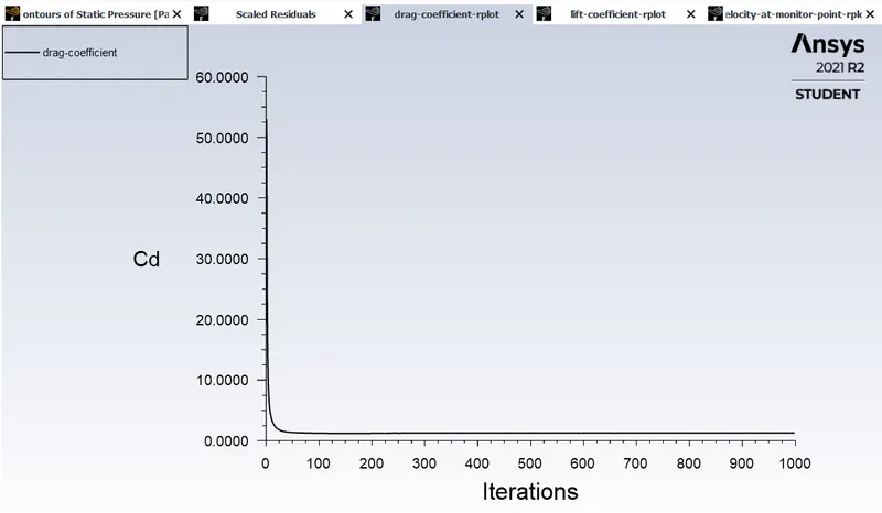
Mean value of drag coefficient is 1.275
Rms value of lift coefficient is 0.069
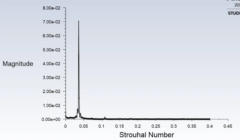
Strouhal number is 0.0359
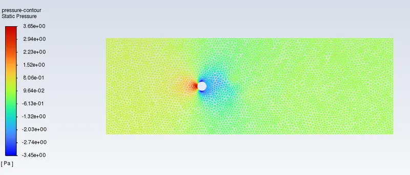
The minimum pressure generated is of value -3.45 Pa
Results -
| S.NO | Solver | Strouhal number | Mean Cd | Rms Cl |
| 1 | Transient | 0.1558 | 1.29 | 0.091 |
| 2 | Steady | 0.0359 | 1.275 | 0.069 |
| 3 | Reference | 0.1569 | 1.3353 | 0.1792 |
| S.NO | Solver | % error absolute | ||
| Strouhal number | Mean Cd | Rms Cl | ||
| 1 | Transient | 0.7 % | 3.39 % | 49.2 % |
| 2 | Steady | 77.11 % | 4.51 % | 61.49 % |
From the table, it is observed that, the results obtained from steady-state solver gives more % error. Since, steady state analysis is time independent, Strouhal number obtained from steady state solver is not accurate compared to transient solver. The error percentage upto 5% is tolerated. The obtained lift coefficient values are not accurate.
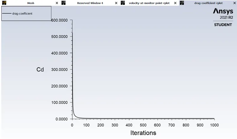
Case 2 - Simulation of flow for Re = 10 - Steady state solver
Velocity at inlet = 0.25 m/s
For Re = 10, no vortex shedding phenomena is not formed.
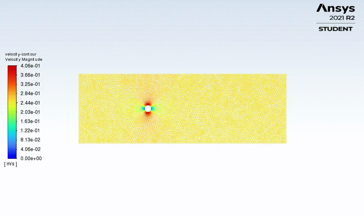
Coefficient of drag - 3.31
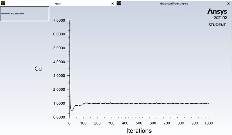
Case 3 - Simulation of flow for Re = 1000 - Steady state solver
Velocity at inlet = 25 m/s
Mean drag coefficient = 0.989
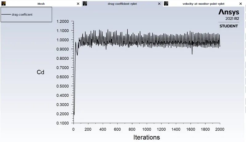
Case 4 - Simulation of flow for Re = 10000 - Steady state solver
Velocity at inlet = 250 m/s
Mean drag coefficient = 0.99
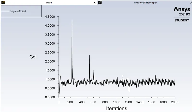
Case 5 - Simulation of flow for Re = 100000 - Steady state solver
Velocity at inlet = 2500 m/s
Mean drag coefficient = 0.8
Results:
The following table shows the mean drag coefficient values obtained for different Reynolds number.
| S.NO | Re | Mean drag coefficient |
| 1 | 10 | 3.31 |
| 2 | 100 | 1.275 |
| 3 | 1000 | 0.989 |
| 4 | 10000 | 0.99 |
| 5 | 100000 | 0.8 |
In laminar flow, the viscous forces dominate inertial forces. The viscous shear forces and pressure forces are primarily responsible for drag force. So, it is observed from the table, as the Reynolds number increases, the effect of viscous forces decreases which causes decrease in drag coefficient.
CONCLUSION:
It is concluded that, results obtained by simulating the flow with transient solver are accurate compared to steady state solver. The effect of drag force decreases as Reynolds number increases.
References -
[1]Rajani, B. N., A. Kandasamy, and Sekhar Majumdar. "Numerical simulation of laminar flow past a circular cylinder." Applied Mathematical Modelling 33.3 (2009): 1228-1247.