Week 2 - Flow over a Cylinder.

Flow over a cylinder

Let us discuss some phenomenon and few numbers before proceeding.

a) Karman Vortex street: Whenever there is bluff (as opposite to streamlined body) in the flow passage of the fluid over it, at certain velocities depending upon shape and size of body, Vorte shedding phenomenon is seen. Its an oscillating flow over bluff body, which forms vortices at back of body and they detatch periodically and forms Karman Vortex street. This street is repetition of swirling vortices and is responsible for unsteady flow separation over a body.

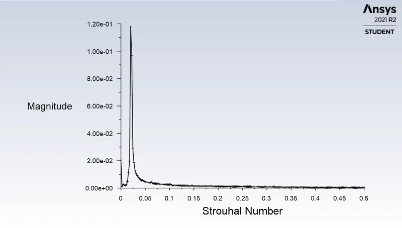
b) Strouhal no. : It is dimensionless number which is important in oscillating flow mechanisms. It is given as below,

Sr = fD/V, where f is vortex shedding frequency, D is characteristic diameter of cylinder, V is fluid flow velocity.

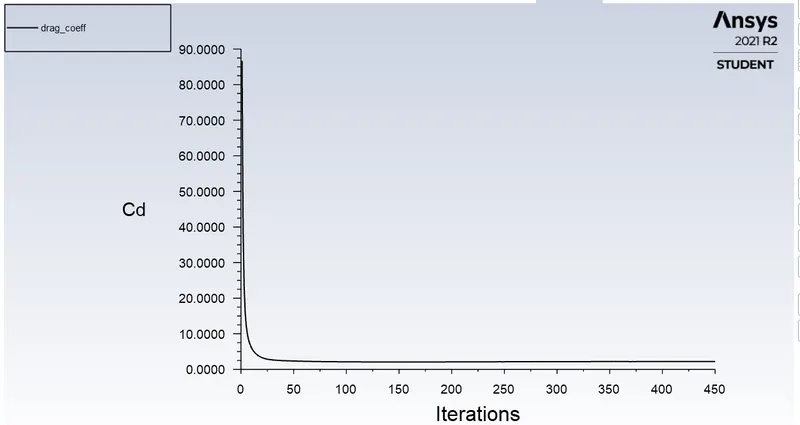
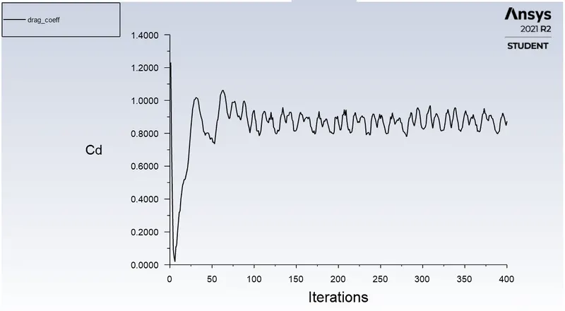
c) Drag coefficient: It is dimensionless quantity which is used to quantify the drag or the resistance of an object in a fluid environment, such as air or water. Lower the value of this quantity means that less resistane the body gives tot he flow.

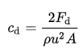
Fd is the drag force, which is component of force in the direction of flow velocity.

Ro is mass density of fluid,

u is flow velocity of the object relative to fluid

A is reference area which is the projected area, in case of car, it is not necessarily the cross section area.

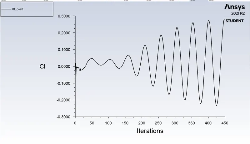
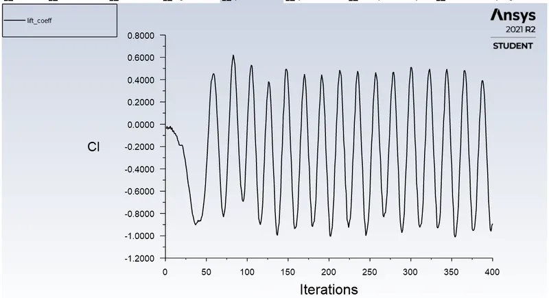
d) Lift coefficient: It is dimensionless quantity that relates the lift generated by the body to the fluid density around the body., fluid velocity and reference area. It is given as,

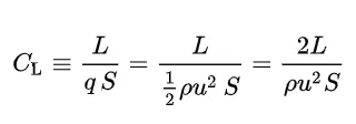
L is lift force,

S is relevent surface area,

q is fluid dymanic pressure

PART 1. Steady and transient simulation for Re = 100

Steady state

step 1: Creating the geometry in OpenClaim

It is created by using line and circle commmand as below,

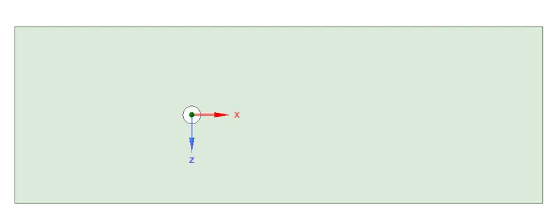
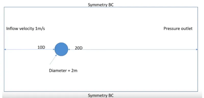
Dimensions of circle is 2m diameter and rectangle flow region is 60*20 m, centre of circle is 20m from inlet.

Step 2: Mesh creation

In meshing, when we create basic mesh, all elemnts are of quad elements, then we change it by adding method insetion and changing it to Tri elements. Then size of element is kept as 0.25m. Also when we looked the mesh around the cylinder surface, we noticed that circle is more looking like polygon with more number of sides. In order to have body fitted mesh , we insert inflation layer near the cylinder wall. First layer height is kept as 5e-3 and growth rate as 1.2 meaning that layer height is increased by 20% after each layer.

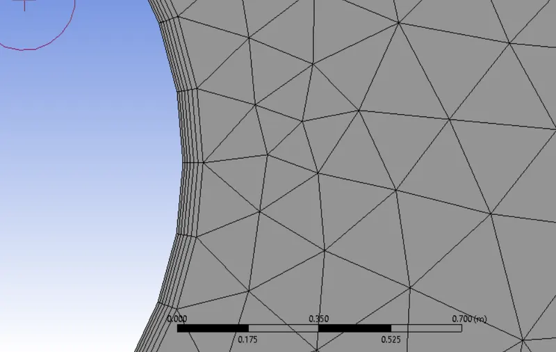
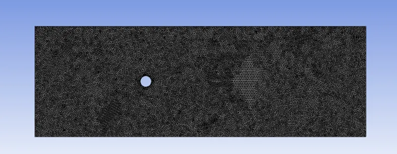
Boundaries are named as below,

Update the mesh.

Step 3: Setting up physics

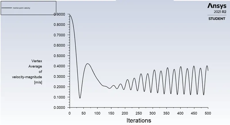
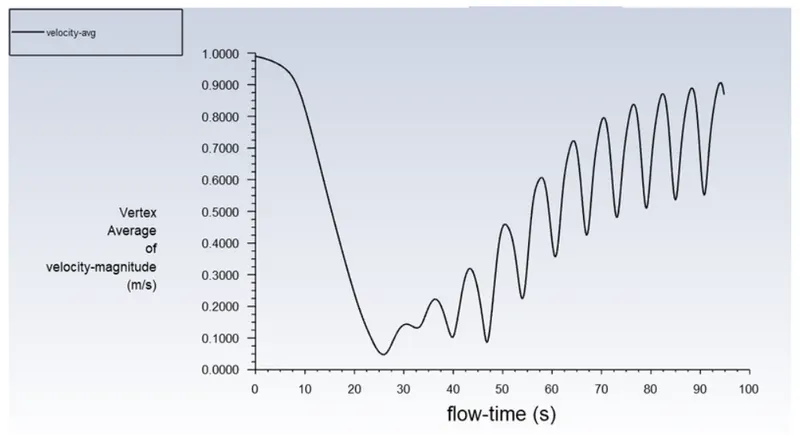
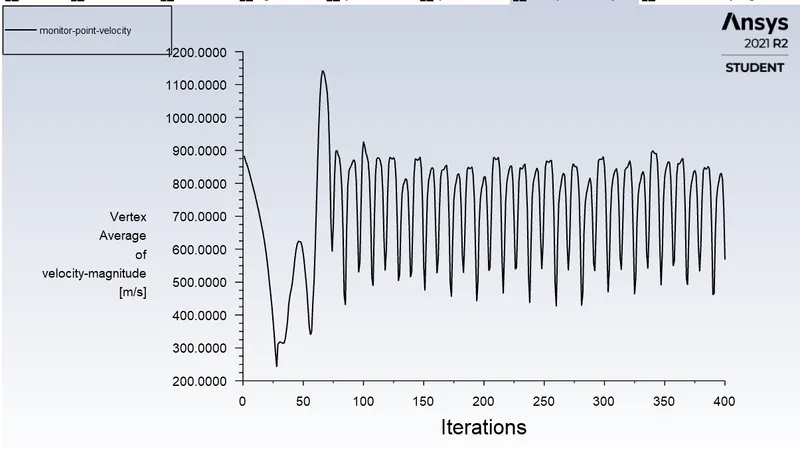
Viscous flow is Laminar. We create the user-Defined material whise density is 1 kg/m3 and kinematic viscosity is 0.02 m2/sec by copying the air and editing it. Then we create monitor point at distance of 8m from inlet. Then create plots for velocity to notice the vortex shedding effect. Use hybrid initialisation for steady state and standard for transient.

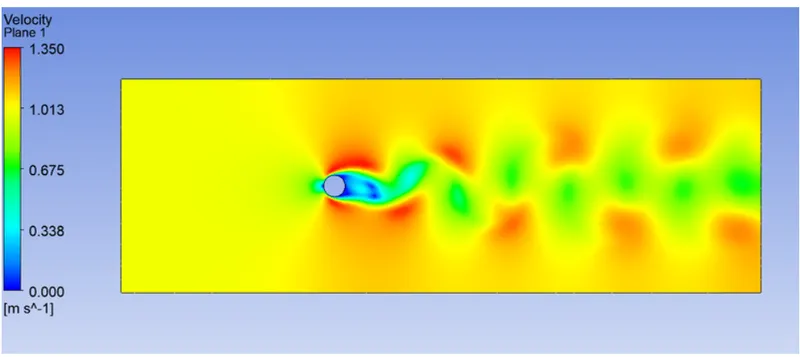
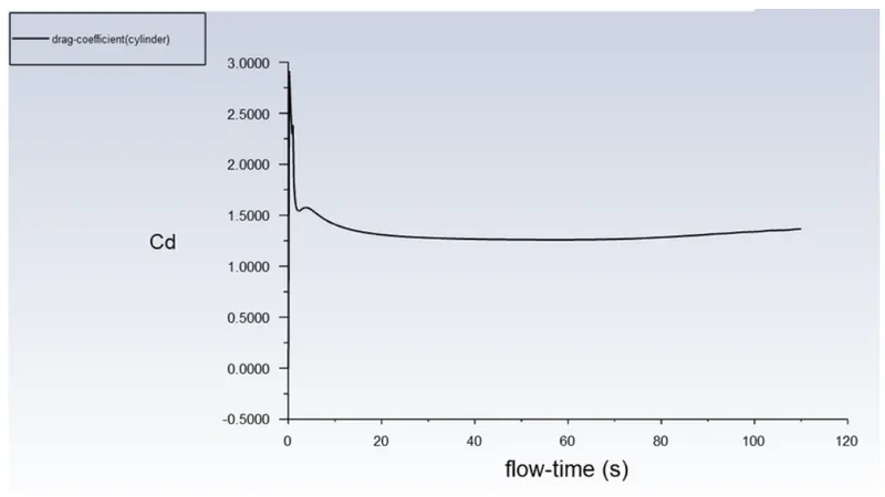
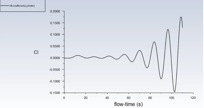
Step 4: Results i) Steady state case for Re = 100, velocity 1 m/s,

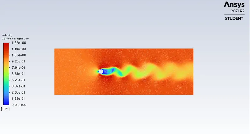
Contour of velocity on surface

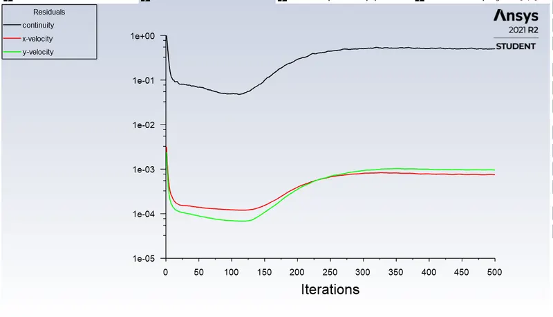
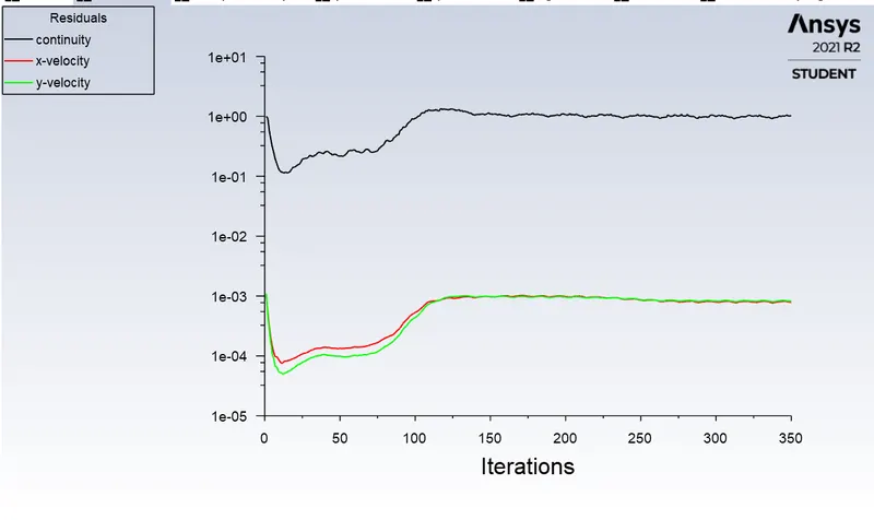
Residual plot

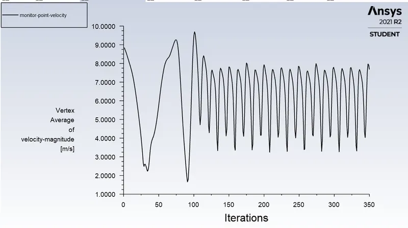
Velocity at monitor point

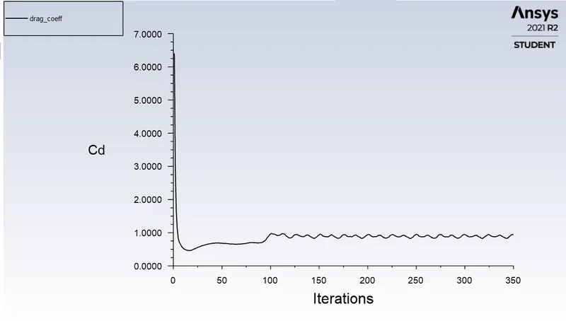
Drag coefficient

Strouhal no.

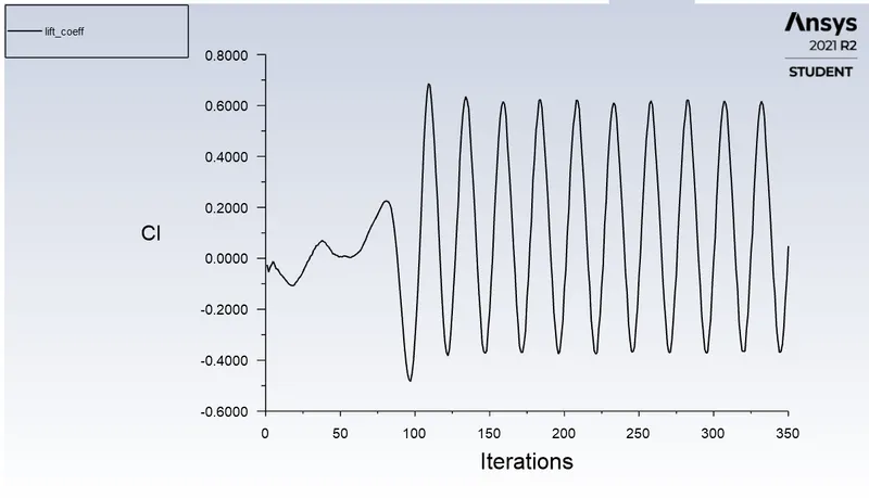
Lift coefficient

ii) Steady state case for Re = 100, velocity 1 m/s,

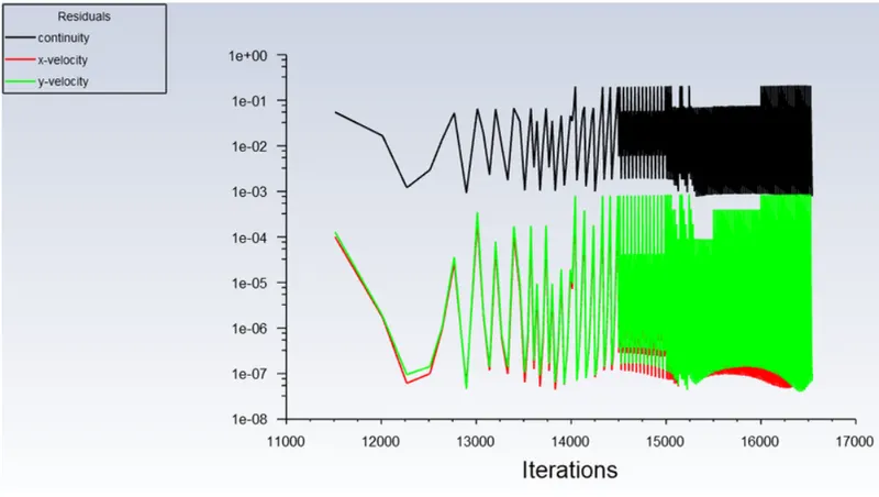
Part 2

Steady flow Re = 10 , V = 0.1 m/s

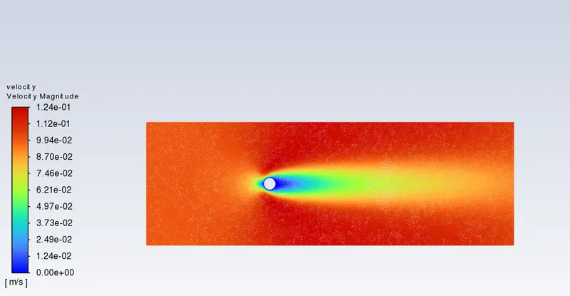
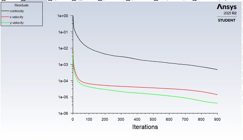
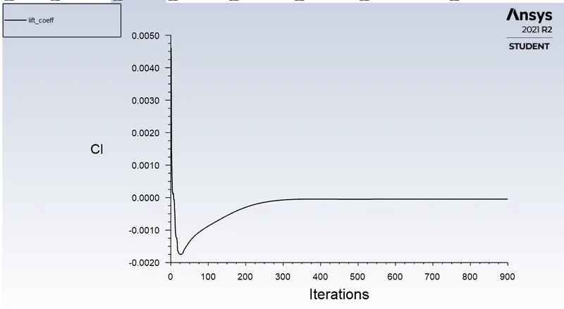
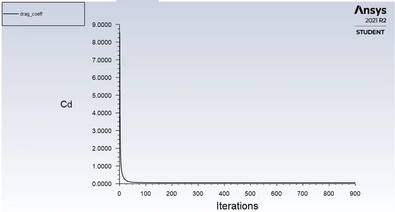
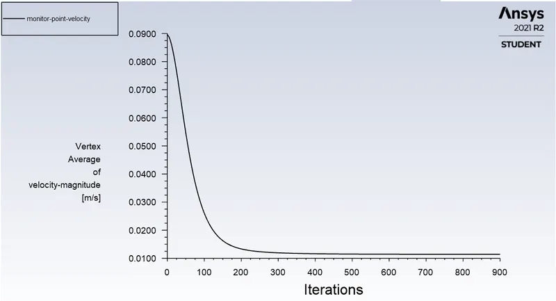
ii) Re = 100

It is done above in part1

iii) Re = 10000, V = 100 m/s

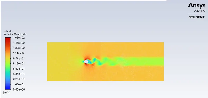
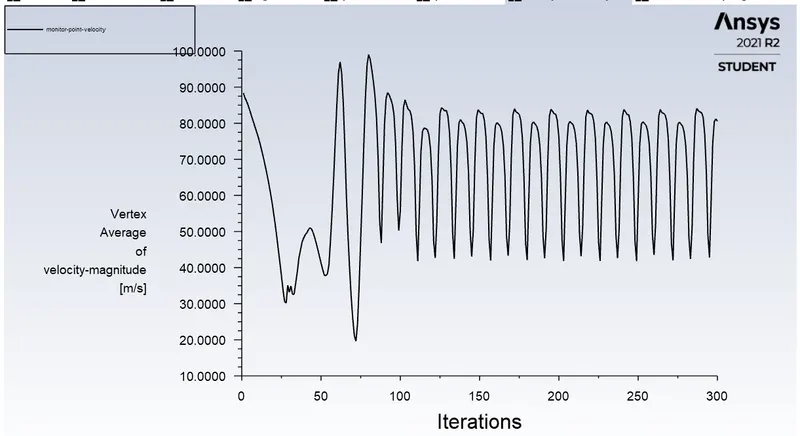
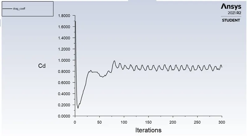
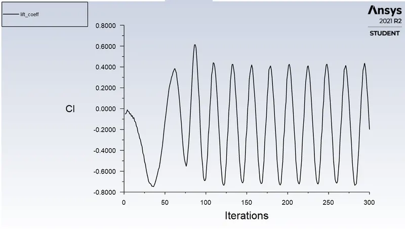
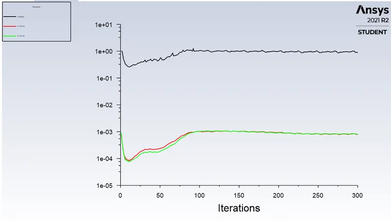
iv) Re = 1000 V= 10 m/s

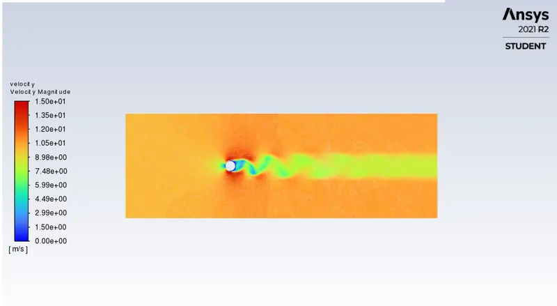
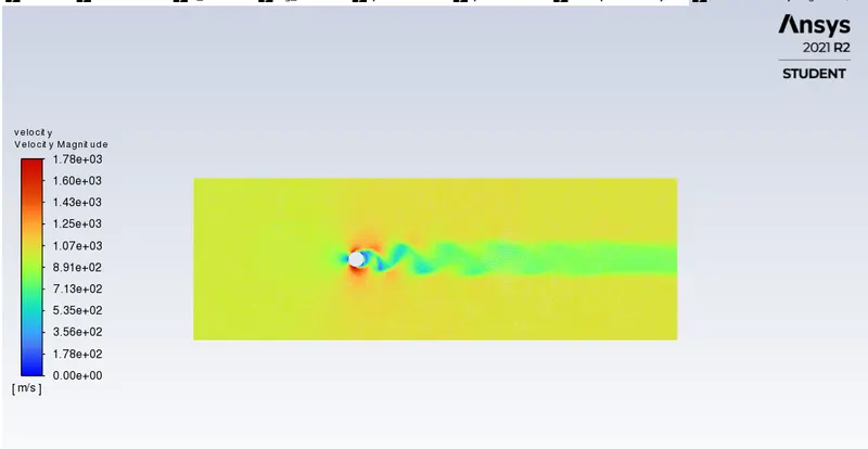
v) Re= 100000 , V = 1000 m/s

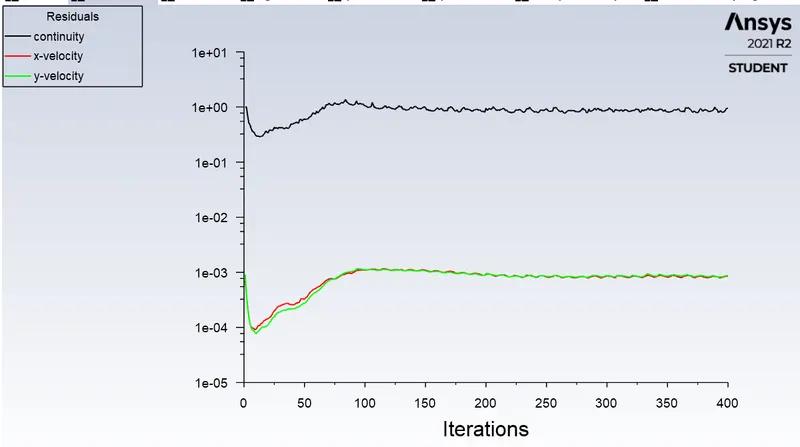
Result:

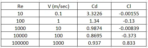
Error wrt theoretical values,

Conclusion:

In the partI, flow over a cylinder is simulated for both steady and transient cases with Re = 100, results are generated and phenomenon of Von Karman vortex street is seen.

In part II, six cases with different Re are simulated to observe behaviour of drag and lift by changing velocity.

In order to observe the behaviour of drag coefficients for the simulations, the velocity of flow is varied to change Reynold's number and rest parameters are kept constant like kinematic viscosity, density.

As we know that Reynold's numbet< 2300, flow is laminar. Hence, we use model as Laminar in viscous model.

In case Re= 10, no vortex shedding is seen. In all rest cases, it is seen.

Also when we refine mesh, the number of elements increases, the no of simulations to converge the solution also increases.

The error percentage is less than or equal to 5% .