Week - 2 - Explicit and Implicit Analysis

AIM: Use the given Equation and Slove using both Explicit and Implicit Methods ( have a tolerence of 10-2).

Given Equation:

F(u) =`u^3``+9u^2+``4u`

How Implicit Analysis Works:

First of all, implicit seems to be a more “basic” solution. In essence it works just as you would think it should!

• Firstly, in each time increment the “global equilibrium” in the model is established. This means that each increment has to converge (this is happening in iterations).

• After global equilibrium is ok, solver calculates all the local finite element variables (stresses etc.) for this increment.

• Benefits: Since global equilibrium is verified at each time increments, those increments can be BIG!
• Drawbacks: Each time increment computes slowly, since iterations are needed to get to the global equilibrium.

How Explicit Analysis Works:

This one is funky. It works in a way, that you don’t have to converge each step! There are no convergence criteria to check and… no iterations! Instead of verifying the “global equilibrium” solver assumes that the equilibrium “simply exists”. This means that the solver goes straight into calculation of local finite element variables! As such procedure has only one step:

• Calculate all of the local finite element variables for given increment, and move to the next one!

• Benefits: Each increment calculates extremely fast!
• Drawbacks: For this to work, the time step has to be EXTREMELY small. Otherwise, it’s impossible to maintain this equilibrium that is assumed to “simply exist”. To achieve this, user do not have direct control over how big-time increments explicit solver will take. Solver itself calculates how small timesteps are still ok. And those acceptable time increments are SUPER SMALL! This is why explicit problems should last fractions of the second! If they would last seconds… you would need millions of increments.

Consider the case of a simple bar in tension as shown in Figure 1. Suppose that the force

in the bar is a nonlinear function of the displacement

F(u) =`u^3``+9u^2+``4u`

From (1) it follows that the stiffffness of the bar is

k(u)=df/du=`3u^2``+18u+``4`

Explicit Analysis:

For this example three equal load increments (or steps) of ∆F = 1unit each are used to load the tension bar. The variables used are u for displacement, f for internal force in the bar, F for external force applied to the bar and k for stiffffness. Incre mental displacements or incremental externally applied forces are represented as ∆u or ∆F, respectively. Use is made of the relationship ∆F = k∆u. The analysis proceeds as follows.

Step1:

`u0=0=>k(u0)=4,Delta F=1,Delta u1= (Delta F)/(k(u0))=1/4=0.25`

`u1=u0+Delta u1=0+0.25=0.25`

Step2:

`u1=0.25=>k(u1)=8.6875,Delta F=1,Delta u2= (Delta F)/(k(u1))=1/8.6875=0.1151`

`u2=u1+Delta u2=0.25+0.1151=0.3651`

Step3:

`u2=0.3651=>k(u2)=10.9716,Delta F=1,Delta u3= (Delta F)/(k(u2))=1/10.9716=0.0911`

`u3=u2+Delta u3=0.3651+0.0911=0.4562`

Finally, from the three steps the following results are obtained.

F external=`Delta F +Delta F+Delta F`=3

f internal(1)=`(0.25)^3+9(0.25)^2+4(0.25)=1.5781`

f internal(2)=`(0.3651)^3+9(0.3651)^2+4(0.3651)=2.7087`

f internal(3)=`(0.4562)^3+9(0.4562)^2+4(0.4562)=3.7928`

It is evident from the results that external and internal forces are NOT in equilibrium because (F external `!=`f internal)

Explicit Analysis
steps	F-external	f-internal	Displacement(u)	R=F-external-F-external
0	0	0	0	0
1	1	1.5781	0.25	0.5781
2	2	2.7081	0.3651	0.7081
3	3	3.7928	0.4562	0.7928

Implicit Analysis:

An implicit analysis is the same as the explicit analysis, except that at the end of each step Newton-Raphson iterations are used to enforce equilibrium before moving to the next step.

However, internal forces and external forces will not be in equilibrium unless the stiffffness is linear for the given step. Hence, in order to achieve equilibrium, corrections must be made to the displacement. This is accomplished by using Newton-Raphson iterations to minimize the residual, R(u) = f internal - F external. Expanding the residual as a Taylor series about the current displacement `u^j` gives

`delta u^(j+1)=-[k(u^j)]^-1 R^j`

Notice that the iteration variable is j and it may take several iterations for the norm of theresidual, ||R ||, to be reduced below the chosen tolerance criteria (10^-2)

Step1:

`u0=0=>k(u0)=4,Delta F=1,Delta u1= (Delta F)/(k(u0))=1/4=0.25`

`u1=u0+Delta u1=0+0.25=0.25`

Check for the residual, F external =`Delta F`=1, F internal=`(0.25)^3+9(0.25)^2+4(0.25)=1.5781`

`R^0=fInternal-Fexternal``=1.5781-1=0.5781`

`||R^0||>10^-2`-newton Raphion iterations necessary.

Caluclate the corection to u1=`u1^(0)`

`delta u^(1)=-[k(u1^(0))]^-1R^(0)=-(8.6875)^-1(0.5781)=-0.0665`

The Updated value of `u1^((1))=u1^((0))+delta u^((1))=0.25-0.0665=0.1835`

Check the residual again;

Fextenal=1,f internal=1.0432

`R^(1)=f Internal-Fexternal=1.0432`

`R^(1)>10^(-2)`

Another iteration is necessary.

Caluclate the total new correction .

`u1=u1^(1)`

`delta u^((2))=delta u^((1))-[k(u1^(1))]^-1R^(1)`

=`-0.0665-(7.4040)^-1(0.0432)`

=`-0.0665-(0.1350)(0.0432)`

=-0.0723

The updated value ;

`u1^((1))=u1^((0))+delta(u)^(2)`

=0.25-0.0723

=0.1777

Check for the residual, fexternal=1, F-internal=`0.1777^3``+9(0.1777)^2+4(0.1777)`

=1.0006

`R^(2)=F Internal-fexternal=1.0006-1`

=0.0006

||`R^((2))||<10^-2`

No iterations are neccessary.

Implcit Analysis
Steps	F-external	f-internal	displacement(u)	R=f-internal-F-external
0	0	0	0	0
1	1	1.0006	0.1777	0.0006
2	2	2.003	0.2965	0.003
3	3	3.0008	0.3911	0.0008

Accurate Solution:

`F(u) =`u^3``+9u^2+``4u``

If F=1;u1=0.1484

If F=2;u2=0.2370

If F=3;u3=0.3062

Accurate solution
Steps	Force	Displacement(u)
0	0	0
1	1	0.1484
2	2	0.237
3	3	0.3062

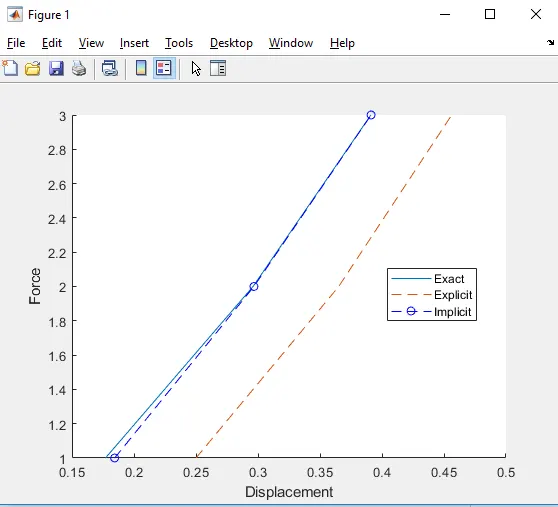
Ploting Graph:

Conclusion:

• As we Observe in the above graph Internal force vs displacement ,Implicit solution and Accurate solution is over laping eachother that means that Implicit solution gives accurate solution than Explicit solution.
• For this to work, the time step has to be EXTREMELY small. Otherwise, it’s impossible to maintain this equilibrium that is assumed to “simply exist”. To achieve this, user do not have direct control over how big-time increments explicit solver will take. Solver itself calculates how small timesteps are still ok. And those acceptable time increments are SUPER SMALL! This is why explicit problems should last fractions of the second! If they would last seconds… you would need millions of increments.