Week - 2 - Explicit and Implicit Analysis

IMPLICIT AND EXPLICIT ANALYSIS REPORT

AIM : To provide a detailed report on implicit and explicit analysis for a given algebraic expression of force acting on a bar as a nonlinear function of displacement.

IMPLICIT VS EXPLICIT SCHEMES (OR) METHODS TO SOLVE NON-LINEAR ANALYSIS :

- The implicit and explicit methods both are used for solving the time dependent structural analysis (or) time-history analysis. Both non-linear static and dynamic problems can be handled with ease.

- STATIC VS DYNAMIC ANALYSIS :

While analysing a problem we need to think about whether the problem is time-dependent (or) time independent. TIme is the main driving factor which helps us to decide about the type of analysis to be chosen.

STATIC ANALYSIS	DYNAMIC ANALYSIS	QUASI-STATIC ANALYSIS
Time independent analysis. The loads are gradually applied over time.	Time dependent analysis and loads applied change with time.	An intermediate case static and dynamic time is taken into account but not the inertial effect.
Inertial effects are negligible and ignored.	Inertial effects taken into account.	Inertial effects are ignored.
APPLICATION : sitting on a chair for longer time (assuming person sitting is still).	APPLICATION : High speed crash impact.	APPLICATION : Low speed crash impact.

- FIELD VARIABLES (OR) THE RESPONSE TO BE CALCULATED FOR STATIC, DYNAMIC AND QUASI-STATIC ANALYSIS :

FIELD VARIABLES (OR) RESPONSE	STATIC ANALYSIS	DYNAMIC ANALYSIS	QUASI-STATIC ANALYSIS
STRESS	YES	YES	YES
STRAIN	YES	YES	YES
DISPLACEMENT	YES	YES	YES
REACTION FORCE	YES	YES	YES
ENERGY	NO	YES	NO
VELOCITY	NO	YES	NO
ACCELERATION	NO	YES	NO
PLASTIC STRAIN	NO	YES	YES
CONTACT PRESSURE	NO	YES	YES

- LINEAR VS NON-LINEAR ANALYSIS :

LINEAR ANALYSIS	NON-LINEAR ANALYSIS
Small deformation(within elastic region)	Large deformation
Material is elastic (Hooke’s Law: $\sigma =E\mathrm{ϵ\; )}$	Material behaviour is plastic
contact point is constant or fixed (fixed boundary conditions)	Contact not fixed

- :

- TYPES OF NON-LINEARITIES IN FEA :

NON-LINEARITY TYPES	DEFINITION
GEOMETRIC NON-LINEARITY	Occurs due to large deformation (or) significant changes in geometry (stiffness changes rapidly)
MATERIAL NON-LINEARITY	Occurs due to the plastic deformation of material
CONTACT (OR) BOUNDARY NON-LINEARITY	Occurs when two surfaces met in contact

- TYPES OF ANALYSIS SOLVED BY METHODS :

ANALYSIS TYPES	METHODS IMPLEMENTED TO SOLVE
Non-linear Static	Implicit approach
Non-linear dynamic	Explicit approach
Quasi-static	Implicit dynamics, implicit and explicit approach

- KEY FORMULATION FOR THE TYPES OF ANALYSIS (OR) GOVERNING EQUATION :

ANALYSIS TYPE	KEY FORMULATION / GOVERNING EQUATION
Static	Ku=F
Dynamic	Mu¨+Cu˙+Ku=F(t)
Quasi-static	K(u)u=F

** F = force applied on the structure, M = mass of the structure , u = displacement (or) deformation of the structure , K = stiffness of the structure , C = damping of the structure

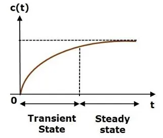
- TRANSIENT VS STEADY VS STEADY STATE RESPONSE :

TRANSIENT RESPONSE	STEADY STATE RESPONSE
Time varying (or) time dependent loads	Time independent loads
Non-equilibrium state	Equilibrium state
Complex computation	Simple computation
Longer simulation time	Shorter simulation time

- KEYWORDS IN FEA:

1. LOAD CONTROL/LOAD STEP : It is the method used to apply/ distribute loads in a controlled manner. In static the load is known i.e, predefined so it is easy for us to control the loads over time and get the responses while in dynamic the load controlled is not known at each instant. These are known as static load control and dynamic load control respectively.

2. TIME-STEP : This explains how the time is incremented to advance the solution for transient dynamic analysis.

3. NUMERICAL STABILITY : This defines to what extent or the degree the numerical accuracy is maintained steadily throughout as the simulation progresses further with very much less error or divergence at each step.

4. ITERATIONS : This is the repeated calculations the solver performs to satisfy the governing equations and constraints.

Now the fundamentals required for the understanding of explicit vs implicit schemes are over. It's time to deep dive into the schemes.

- IMPLICIT VS EXPLICIT SCHEMES IN DETAIL :

* IMPLICIT SCHEME (OR) METHOD :

- This method is mostly for used for non-linear static problems with non - linearities of material, geometry and boundary conditions,

- The current and the previous values are known for solving the system of equations for solving the next time step,

- This method is unconditionally stable because the numerical stability does not depend on any conditions to satisfy the governing equations and constraints,

- Larger time steps are allowed for numerical stability,

EULER BACKWARD METHOD FOR IMPLICIT APPROACH :

u(n+1) = u(n)+Δt⋅f(u(n+1)

where , u ----> displacement (unknown (or) field variable to be calculated),

n ----> initial time step (first),

n+1 -----> second time step succeeding the initial time step 'n',

u(n) ----> initial displacement at time step 'n',

u(n+1) ----> displacement at time step 2 to be calculated using displacement at time step 'n'

Δt -----> time step.

This procedure of method is repeatedly done over again and again till the residual values are obtained or till it satisfies the convergence criteria using "Newton-Raphson method".

* EXPLICIT SCHEME (OR) METHOD :

- This method is mostly for used for non-linear transient dynamic problems with non - linearities of material, geometry and boundary conditions,

- Values from the previous time step are enough to calculate the new values or field variables,

- This method is conditionally stable because the numerical stability depends on conditions to satisfy the governing equations and constraints,

***CONDITION : The time step must be smaller than a elastic wave to propagate from one part of the element to other.

Δt ≤ L/c (for 1d scheme)

, where, L = smallest element length of mesh sizing, c = wave speed (depends on material).

The formulation is given by "COURANT-FRIEDRICHS-LEWY CRITERION (CFL CRITERION)".

** The material properties young's modulus and density affects the wave speed of the material.

- Larger time steps affect the numerical stability thus causing inaccuracy and divergence throughout simulation.

- This method is fast at smaller time step considering the fact that Δt is smaller.

EULER BACKWARD METHOD FOR EXPLICIT APPROACH :

u(n+1) = u(n)+Δt⋅f(u(n) )

** The only difference from that of implicit method is that the time step are controlled and thus makes the simulation conditionally stable for maintaining numerical stability.

- COMMON CONVERGENCE CRITERIA FOR NON-LINEAR STATIC ANALYSIS :

* FORCE CONVERGENCE CRITERIA : The difference between the force applied and the internal force generated due to applied force must be approximately equal to zero.

RESIDUAL FORCE : FORCE APPLIED - INTERNAL FORCE GENERATED DUE TO THE APPLIED FORCE ~ 0. As long as these residual force approaches zero, it can be concluded that body is in static equilibrium.

* DISPLACEMENT CONVERGENCE CRITERIA : This gives the updated values of displacements between each iteration and must be very small for more accuracy. More stiffer is the structure lesser will be the displacement/deformation and it becomes simpler to compute through iterations.

---

- PROBLEM : GIVEN FUNCTION - F(u) = u³+9u²+4u

TYPE OF ANALYSIS TO BE PERFORMED : "NON-LINEAR STATIC ANALYSIS OF A SIMPLE BAR IN TENSION DUE TO APPLIED FORCE F"

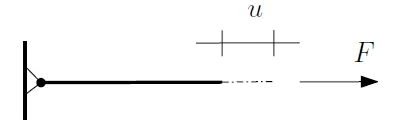
The bar is fixed at one side and the other side of the bar is axially pulled by the force F . Let u be the displacement of the bar along the direction of the applied load F.

The force F given in the bar is a nonlinear function of displacement : f(u) = u3+9u2+4u ----- EQUATION 1

If f(u) is differentiated , k(u) can be obtained ----> k(u) = dF(u)/du = 3u2+18u+4 where k(u) = stiffness of the bar ------ EQUATION 2

- SOLVING THE PROBLEM THROUGH EXPLICIT METHOD : Here the method of incremental explicit load scheme is used which means the load applied is incremented in step by one unit.

For example : here we will take the first three values and we will find the corresponding solution of u at each load incremental step.

STEP -1 : at u0 = 0, k(u0 ) = 4, ΔF = 1 , Δ u1 = ΔF / k(u0 ) = 0.25, u1 = u0 + Δ u1 = 0.25

STEP -2 : k(u1 ) = 4.06 ΔF = 1 , Δ u2 = ΔF / k(u1 ) = 0.24, u2 = u1 + Δ u2 = 0.49

STEP -3 : k(u2 ) = 4.24 ΔF = 1 , Δ u3 = ΔF / k(u2 ) = 0.23, u3 = u2 + Δ u3 = 0.72

STEP-4 : Fext = ΔF + ΔF + ΔF = 3

STEP-5 : fint = u3+9u2+4u at u1 = 1.57 , fint = u3+9u2+4u at u2 = 4.23, fint = u3+9u2+4u at u3 = 7.91

STEP-6 : force convergence criteria failed for the three values analytically but may or may not fail upon further iterations and it can be calculated using "MATLAB".

STEP-7 : It can be concluded that fint not equal to Fext

STEP-8 : Table for residual forces computed analytically

FORCE EXTERNAL	FORCE INTERNAL	RESIDUAL FORCE (R = F(INT) - F(EXT))
1	1.57	0.57
2	4.23	2.23
3	7.91	4.91

- SOLVING THE PROBLEM THROUGH IMPLICIT METHOD : This method also follow the same as of explicit except before going to next iteration the values are iterated using Newton raphson method.

From the residual values calculated before at u0=0 R was 0.57 which is more than 0.01 which implies that newton raphson iteration is necessary. Now calculate the new correction U1 =0.14

new value of u = u(1) + U(1) = 0.25 + (-0.14) = 0.11 which is greater than 0.01 so we need to implement again newton raphson for further accuracy. Follow the saem to achieve accuracy but we can see that 1 to 3 iterations are enough

to get the achieved equilibrium state .

- Final Plot of force vs displacement using explicit,implicit and exact method :

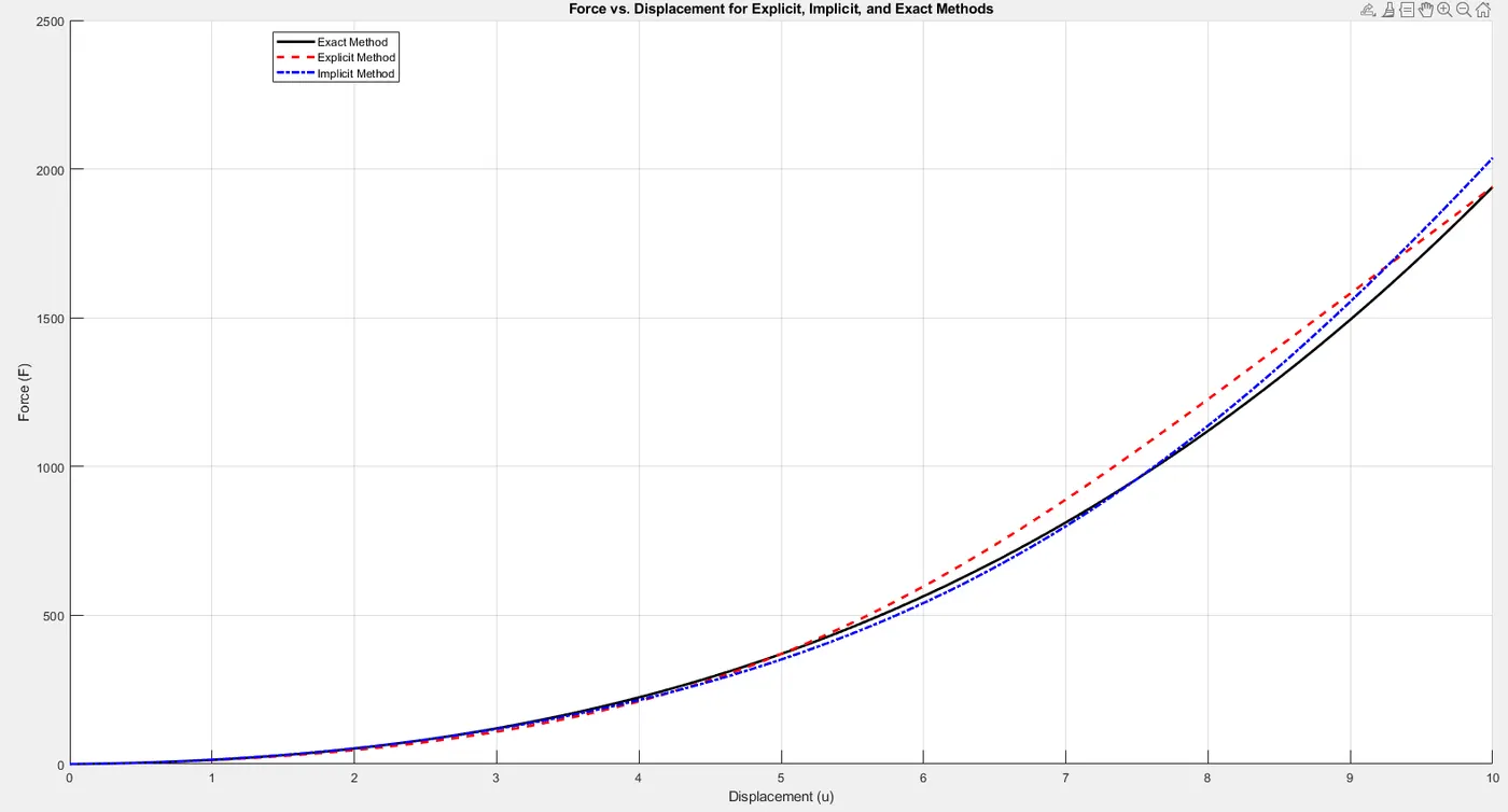
CONCLUSION : From the above graph it can be seen that the implicit method overcome the problem of maintain a stable equilibrium throughout simulation even though it has deviations from the exact but results almost same to that of the exact values. The explicit methods was less approximate to that of the exact value for this non-linear static analysis. At the end, the most useful load incremental scheme was the implicit one using Newton Raphson method and tolerance of 0.01 has been maintained throughout.