Week - 2 - Explicit and Implicit Analysis

Aim : To solve the given problem using both explicit and implicit method and plotting the results. It shows an example nonlinear static problem. In both cases an incremental load control scheme is used.

Consider the case of a simple bar in tension. Suppose that the force in the bar is a nonlinear function of the displacement.

f(u)=u³+9u²+4u …………(1)

F(u) = u³ +9u² + 4u

Stiffness, k(u)= dF(u)/ du = 3u²+ 18u + 4 ………….(2)

Explicit analysis

Clearly it is possible to plot a graph of force, f, versus displacement, u, by using equation (1). However, if the nonlinear force versus displacement relationship is not known, but the stiffness is known, it is possible to construct the graph of force versus displacement numerically. One method is to use an incremental explicit load control scheme. This is illustrated next. For this example, three equal load increments (or steps) of ∆F = 1 unit each are used to load the tension bar. The variables used are u for displacement, f for internal force in the bar, F for external force applied to the bar and k for stiffness. Incremental displacements or incremental externally applied forces are represented as ∆u or ∆F, respectively. Use is made of the relationship ∆F = k∆u. The analysis proceeds as follow

Force function, F(u) = (u)³+ 9(u)² + 4u

Displacement = Force/Stiffness = F/k

Force increment = dF = 1

Displacement increment, du = dF/k

Displacement, u_i+1 =u_i + du_i

Step 1:

dF = 1

k(u₀) = 3(u₀)² + 18u₀ + 4 = 3.0² + 18.0+ 4 = 4

du₁ =dF/ k(u₀) = ¼ = 0.25

u₁= u₀ + du₁ = 0 + 0.25 = 0.25

F(u₁) = (u₁)³ + 9(u₁)²+ 4u₁ = 0.25³ + 9. 0.25² + 4.0.25 = 1.578

F_ext= dF = 1

u_exact= 0.177 { by solving the equation. F_ext= (u_exact)³ + 9(u_exact)²+ 4u_exact }

Step 2:

dF = 1

k(u₁) = 3(u₁)² + 18u₁ + 4 = 3*0.25² + 18*0.25 + 4 = 8.688

du₂ =dF/ k(u₁) = 1/8.688 = 0.115

u₂ = u₁ + du₂ = 0.25 +0.115 = 0.365

F(u₂) = (u₂)³ + 9(u₂)²+ 4u₂ = 0.365³ + 9* 0.365² + 4*0.365 = 2.709

Ft = dF + dF = 1+1 = 2

u_exact= 0.296 { by solving the equation. F_ext= (u_exact)³ + 9(u_exact)²+ 4u_exact }

Step 3:

dF =1

k(u₂) = 3(u₂)² +18 u₂ + 4 = 3*0.365² + 18*0.365 +4 = 10.972

du₃ = dF/k(u₂) = 1/10.972 = 0.091

u₃ = u₂ + du₃ = 0.365 + 0.091 = 0.456

F(u₃) = (u₃)³ + 9(u₃)² + 4 u₃ = 0.456³ + 9*0.456²+ 4*0.365 = 3.793

F_ext= dF + dF + dF =1+1+1 = 3

u_exact= 0.391 { by solving the equation. F_ext= (u_exact)³ + 9(u_exact)²+ 4u_exact }

It is evident from the results that external and internal forces are not in equilibrium because F_ext = f_int. Table summarizes the main results for the explicit analysis.

step i	∆Fi	∆ui	ui	(Fext)i	(fint)i	Fext - fint = R
1	1.0	0.25	0.115	1	1.578	0.578
2	1.0	0.115	0.365	2	2.709	0.709
3	1.0	0.091	0.456	3	3.793	0.793

Implcit analysis

An implicit analysis is the same as the explicit analysis, except that at the end of each step Newton-Raphson iterations are used to enforce equilibrium before moving to the next step. Basically, an incremental force is applied to advance the solution forward at the beginning of a step. However, internal forces and external forces will not be in equilibrium unless the stiffness is linear for the given step. Hence, in order to achieve equilibrium, corrections must be made to the displacement. This is accomplished by using Newton-Raphson iterations to minimize the residual, R(u) = fint − Fext. Expanding the residual as a Taylor series about the current displacement u^j gives

R^j+1 = R^j(u^j) + (dR(u^j)/du)ẟu^j+1 +…R^j + k(u^j)ẟu^j+1 +…

By neglecting higher-order terms in the series, setting R^j+1 = 0 and solving for ẟu^j+1 , the following correction is obtained:

ẟu^j+1 = -[k(u^j)]^-1 R^j

Notice that the iteration variable is j and it may take several iterations for the norm of the residual, ||R || to be reduced below the chosen tolerance criteria (0.01 in this case). The implicit analysis proceeds as follows:

Force function, F(u) = (u)³ + 9(u)² + 4u

Stiffness, k(u) = dF(u)/du = 3u² + 18u + 4

Displacement = Force/Stiffness = F/k

Force increment = dF =1

Displacement increment, du= dF/k

Displacement, u_i+1 = u_i + du_i

Step 1:

dF = 1

k(u₀) = 3(u₀)² + 18u_0­­­ + 4 = 3*0² + 18*0 + 4 = 4

du₁ = dF/k(u₀)=1/4 = 0.25

u₁= u₀+du₁=0 + 0.25 = 0.25

F(u₁) = (u₁)³ +9(u₁)²+ 4u₁= 0.25³ + 9* 0.25² + 4* 0.25 = 1.578

F_ext = dF = 1

R=F(u₁) – F_ext = 1.000 = 0.578

||R|| >0.01. Therefore, Newton-Raphson iterations have to be done to obtain a correction factor that will bring the Value within our tolerance limit.

iteration 1:

u₁⁽⁰⁾ = u₁ = 0.25

Correction factor for u₁ = ẟu₁⁽¹⁾ = -[k(u₁⁽⁰⁾)]^-1R⁽⁰⁾

K(u₁⁽⁰⁾) = k(u₁) = 3*0.25² + 18*0.25 + 4 = 8.688

R⁽⁰⁾ = 0.578

ẟu₁⁽¹⁾ = -[k(u₁⁽⁰⁾)]^-1R⁽⁰⁾ = -[8.688]^-1*0.578= -0.06653

Corrected u₁ = u₁⁽¹⁾ + ẟu₁⁽¹⁾ = 0.25 +(-0.06653) = 0.183

F⁽¹⁾ = (u₁⁽¹⁾)³ + 9(u₁⁽¹⁾)² + 4 u₁⁽¹⁾

= 0.183³ + 9*0.183 + 4 *0.183 = 1.039

Updated Residual, R⁽¹⁾ = F⁽¹⁾ – F_ext = 1.039 – 1 = 0.039

||R|| > 0.01. Proceed to the next iteration as ||R|| is not within the tolerance limit.

Iteration 2.

Correction factor for u₁ = ẟu₁⁽²⁾ = ẟu₁⁽¹⁾ = -[k(u₁⁽¹⁾)]^-1R⁽¹⁾

K(u₁⁽¹⁾) = k(u₁) = 3*0.183² + 18*0.183 + 4 = 7.394

R⁽¹⁾ = 0.039

ẟu₁⁽²⁾ = ẟu₁⁽¹⁾ = -[k(u₁⁽¹⁾)]^-1R⁽¹⁾ = -0.06653-[7.394]^-1*0.039= -0.0718

Corrected u₁ = u₁⁽²⁾ = u₁ + ẟu₁⁽²⁾ = 0.25 +(-0.0718) = 0.1782

F⁽²⁾ = (u₁⁽²⁾)³ + 9(u₁⁽²⁾)² + 4 u₁⁽²⁾

= 0.1782³ + 9*0.1782² + 4 *0.1782 = 1.004

Updated Residual, R⁽²⁾ = F⁽²⁾ – F_ext = 1.004 – 1 = 0.004

||R|| < 0.01. ||R|| has reached within the tolerance limit. Thus, no need for further iterations.

Therefore, F(u₁) = F(u₁⁽²⁾) = 1.004 and the final corrected value of u₁ = u₁⁽²⁾ = 0.1782

STEP 2:

dF = 1

k(u₁) = 3(u₁)² + 18u_1­­ + 4 = 3*0.1782² + 18*0.1782 + 4 = 7.302

du₂ = dF/k(u₁)=1/7.302 = 0.137

u₂= u₁+du₂ = 0.1782 + 0.137 = 0.315

F(u₂) = (u₂)³ +9(u₂)²+ 4u₂= 0.315³ + 9* 0.315² + 4* 0.315 = 2.184

F_ext = dF + dF = 1 + 1 = 2

R=F(u₂) – F_ext = 2.184 - 2.000 = 0.184

||R|| >0.01. Therefore, Newton-Raphson iterations have to be done to obtain a correction factor that will bring the Value within our tolerance limit.

Iteration 1:

u₂⁽⁰⁾ = u₂

Correction factor for u₂ = ẟu₂⁽¹⁾ = -[k(u₂⁽⁰⁾)]^-1R⁽⁰⁾

K(u₁⁽⁰⁾) = k(u₁) = 9.967

R⁽⁰⁾ = 0.184

ẟu₂⁽¹⁾ = -[k(u₂⁽⁰⁾)]^-1R⁽⁰⁾ = -[9.967]^-1*0.184= -0.0185

Corrected u₂ = u₂⁽¹⁾ = u₂ + ẟu₁⁽¹⁾ = 0.315 +(-0.0185) = 0.296

F⁽¹⁾ = (u₂⁽¹⁾)³ + 9(u₂⁽¹⁾)² + 4 u₂⁽¹⁾

= 0.296³ + 9*0.296 + 4 *0.296 = 1.998

Updated Residual, R⁽¹⁾ = F⁽¹⁾ – F_ext = 1.998 – 2 = -0.002

||R|| < 0.01. ||R|| has reached within the tolerance limit. Thus, no need for further iterations.

Therefore, F(u₂) = F(u₂⁽¹⁾) = 1.998 and the final corrected value of u₂ = u₂⁽¹⁾ = 0.296

STEP 3:

dF = 1

k(u₂) = 3(u₂)² + 18u_2­­ + 4 = 3*0.296² + 18*0.296 + 4 = 9.59

du₃ = dF/k(u₂)=1/9.59 = 0.104

u₃= u₂+du₃ = 0.296 + 0.104 = 0.4

F(u₃) = (u₃)³ +9(u₃)²+ 4u₃= 0.4³ + 9* 0.4² + 4* 0.4 = 3.104

F_ext = dF + dF + dF = 1 + 1 + 1 = 3

R=F(u₃) – F_ext = 3.104 - 3.000 = 0.104

||R|| >0.01. Therefore, Newton-Raphson iterations have to be done to obtain a correction factor that will bring the Value within our tolerance limit.

Iteration 1.

u₃⁽⁰⁾ = u_{3 = 0.4}

Correction factor for u₃ = ẟu₃⁽¹⁾ = -[k(u₃⁽⁰⁾)]^-1R⁽⁰⁾

k(u₃⁽⁰⁾) = k(u₃) = 11.68

R⁽⁰⁾ = 0.104

ẟu₃⁽¹⁾ = -[k(u₃⁽⁰⁾)]^-1R⁽⁰⁾ = -[11.68]^-1*0.104= -0.0089

Corrected u₃ = u₃⁽¹⁾ = u₃ + ẟu₃⁽¹⁾ = 0.4+(-0.089) = 0.3911

F⁽¹⁾ = (u₃⁽¹⁾)³ + 9(u₃⁽¹⁾)² + 4 u₃⁽¹⁾

= 0.39911³ + 9*0.3911 + 4 *0.3911 = 3.0008

Updated Residual, R⁽¹⁾ = F⁽¹⁾ – F_ext = 3.0008 – 3 = 0.0008

||R|| < 0.01. ||R|| has reached within the tolerance limit. Thus, no need for further iterations.

Therefore, F(u₃) = F(u₃⁽¹⁾) = 3.0008 and the final corrected value of u₃ = u₃⁽¹⁾ = 0.3911

The results of the implicit analysis are summarized in Table. It is evident from the table that the external forces and internal forces are coming into equilibrium.

Step i	∆Fi	ui	(Fext)i	(fint)i	Fext - fint = R
1	1.0	0.250	1	1.0043	0.0043
2	1.0	0.365	2	1.9985	-0.0015
3	1.0	0.456	3	3.0009	0.0009

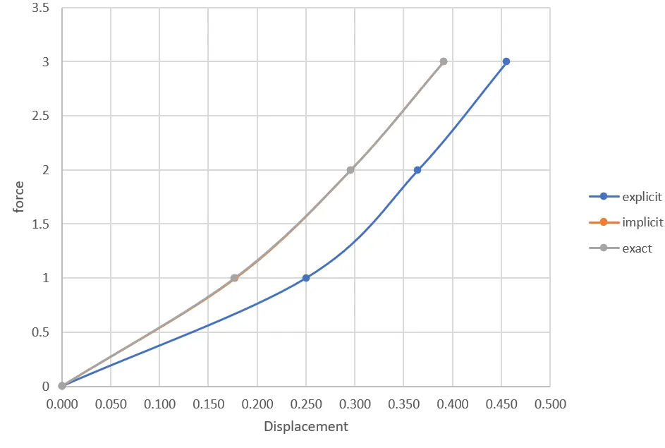
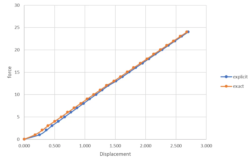
A plot of the results is shown in Figure. It is evident from the plot that the explicit analysis drifts from the exact solution. If 20 increments are used the explicit analysis more closely follows the exact solution as shown. However, even with more increments the explicit analysis still drifts from the exact solution. The drift from the exact solution illustrates the lack of equilibrium between the internal and external forces. To correct for this problem an implicit analysis is required. The results for the implicit analysis are shown. The Newton-Raphson iterations correct the incremental steps so that they land on the exact solution according to the specified tolerance. Excellent agreement is achieved with just 3 increments and in each step only two Newton-Raphson iterations are required. The explicit and implicit analyses are completed by using simple MATLAB scripts.

Conclusion:

A nonlinear analysis is illustrated using an incremental explicit and implicit procedure. The results are plotted for comparison. It is evident from the results that the explicit analysis drifts from the true solution. To overcome this problem an implicit analysis is used, which includes Newton-Raphson iterations to enforce equilibrium between internal and external forces. The techniques demonstrated are for a load control scheme. Many of the concepts and methods introduced are similar to concepts and methods used in a nonlinear finite element analysis. Therefore, the given example is a useful for learning about methods of solution for nonlinear problems.