Week - 2 - Explicit and Implicit Analysis

Aim:

To solve the given equation F(u) = u3+9u2+4u using both explicit and implicit methods (with a tolerance of 0.001)

Explicit and implicit methods:

Explicit and implicit methods are numerical analaysis methodologies used for obtaining numerical approximations to the solutions of time-dependent ordinary and partial differential equations. Explicit methods are used to calculate the state of the system at a later time from the state of the system at the current time.

x(n+1) = x(n)+ z(n)

Implicit methods are used to find a solution both the current state of the system and the later one.

x(n+1) = x(n)+z(n+1)

The explicit method is easier to program and can be calculated within a shorter time. The stability of explicit method is so low that a smaller step size to prevent divergence. Meanwhile, the implicit method has high stability and converges if proper parameters are set. But, since equations has to be solved at every step, it can take longer time to calculate.

The implicit methods can use a sufficiently large step size. Hence, it is suitable for solving equations that involve a long time. Also, in non-linear equations such as contact, it is difficult to predict a future from the past state. Therefore, in these cases, implict method is used than the explicit method.

Calculation:

F(u) = u3+9u2+4u --> (1)

The stiffness k(u) = 3u2+18u+4 --> (2)

Explicit analysis:

Step 1:

Take u0 = 0.0 => k(u0) = 4, ΔF = 1, Δu1 = ΔF/k(u0) = 1/4 = 0.25; u1 = u0 + Δu1 = 0.0 + 0.25 = 0.25

Step 2:

=> k(u1) = 3(u1)² + 18 (u1) + 4 = 3 (0.25)² + 18 (0.25) + 4 = 0.1875 + 4.5 + 4 = 8.6875; ΔF = 1, Δu2 = ΔF/k(u1) = 1/8.6875 = 0.1151; u2 = u1 + Δu2 = 0.25 + 0.1151 = 0.3651

Step 3:

=> k(u2) = 3(u2)² + 18 (u1) + 4 = 3 (0.3651)² + 18 (0.3651) + 4 = 0.3998 + 6.5718 + 4 = 10.9716; ΔF = 1, Δu3 = ΔF/k(u2) = 1/10.9716 = 0.0911; u3 = u2 + Δu3 = 0.3651 + 0.0911 = 0.4562

Finally, from the three steps the following results are obtained:

F(ext) = ΔF + ΔF + ΔF = 3.0

f(int) = u3³+9u3²+4u3 = (0.4562)³ + 9(0.4562)² + 4(0.4562) = 0.0949 + 1.8730 + 1.8248 = 3.7927

It is evident from the results that external and internal forces are NOT in equilibrium because F(ext)≠f(int).

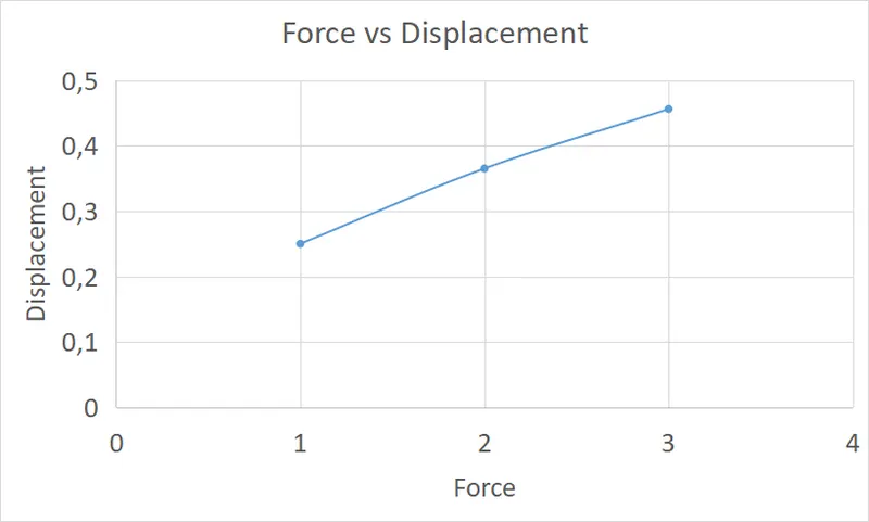
The main results for the explicit analysis are as follows:

Step i	ΔFi	ui	Δui	F(ext)i	f(int)i	f(int)-F(ext) = R
1	1.0	0.25	0.25	1.0	1.5781	0.5781
2	1.0	0.3651	0.1151	2.0	2.7087	0.7087
3	1.0	0.4562	0.0911	3.0	3.7927	0.7927

Implicit analysis:

Step 1:

u0 = 0.0 => k(u0) = 4, ΔF = 1, Δu1 = ΔF/k(u0) = 1/4 = 0.25; u1 = u0 + Δu1 = 0.0 + 0.25 = 0.25

Check the residual, F(ext) = ΔF = 1, f(int) = u1³+9u1²+4u1 = 1.5781, R(0) = f(int)-F(ext) = 1.5781 - 1 = 0.5781

||R(0)||> 0.01 => Newton-Raphson iterations are necessary

• Calculate the correction to u1 = u1(0)
  δu1 = -[k(u1(0)]^-1.R(0) = -([3(0.25)²+18(0.25)+4]^-1)*0.5781 = -((0.1875+4.5+4)^-1)*0.5781 = -0.0665
  
  • The updated value of u1(1) = u1(0) + δu1 = 0.25-0.0665 = 0.1835
    Check the residual again, F(ext) = 1, f(int) = (u1(1))³+(9u1(1))²+4u1(1) = (0.1835)³ + (9*(0.1835)²)+ 4*(0.1835) = 0.0061+0.3030+0.734 = 1.0431
    R(1) = f(int) - F(ext) = 0.0431
    ||R(1)||> 0.01 => Newton-Raphson iterations are necessary
• Calculate the new total correction to u1 = u1(0)
  δu2 = δu1 - [k(u1(1)]^-1.R(1) = -0.0665 -([3(0.1835)²+18(0.1835)+4]^-1)*0.0431 = -0.0665-((0.1010+3.303+4)^-1)*0.0431 = -0.0665 -0.0058 = -0.0723
  • The updated value of u1(2) = u1(0) + δu2 = 0.25 + (-0.0723) = 0.1777
    Check the residual, F(ext) = 1, f(int) = (u1(2))³+9(u1(2))²+4u1(2) = (0.1777)³+9(0.1777)²+4(0.1777) = 0.0056+0.2841+0.7108 = 1.0005
    R(2) = f(int) - F(ext) = 0.0005
    ||R(2)||< 0.01 => no further iterations are necessary
• Therefore, the final value is u1 = u1(2) = 0.1777

Step 2:

k(u1) = 3(0.1777)²+18(0.1777) +4 = 0.0947 + 3.1986 + 4 = 7.2933, ΔF = 1, Δu2 = ΔF/k(u1) = 1/7.2933 = 0.1371

u2 = u1 + Δu2 = 0.1777+0.1371 = 0.3148

Check the residual, F(ext) = ΔF = 1, f(int) = u2³+9u2²+4u2 = (0.3148)³ + 9(0.3148)² + 4(0.3148) = 0.0311 + 0.8918 + 1.2592 = 2.1821, R(0) = f(int) - F(ext) = 2.1821 - 2 = 0.1821

||R(0)||> 0.01 => Newton-Raphson iterations are necessary

• Calculate the correction to u2 = u2(0)
  δu1 = -[k(u2(0)]^-1.R(0) = -([3(0.3148)²+18(0.3148)+4]^-1)*0.1821 = -((0.2972+5.6664+4)^-1)*0.1821 = -0.01827
  • The updated value of u2(1) = u2(0) + δu1 = 0.3148-0.01827 = 0.2965
    Check the residual again, F(ext) = 1, f(int) = u2(1)³+9u2(1)²+4u2(1) = (0.2965)³+9(0.2965)²+4(0.2965) = 0.0260+0.7912+1.186 = 2.0032
    R(1) = f(int) - F(ext) = 0.0032
    ||R(1)||< 0.01 => no further iterations are necessary
• Therefore, the final value of u2 = u2(1) = 0.2965

Step 3:

k(u2) = 3(0.2965)²+18(0.2965) +4 = 0.2637 + 5.337 + 4 = 9.6007, ΔF = 1, Δu3 = ΔF/k(u2) = 1/9.6007 = 0.1041

u3 = u2 + Δu3 = 0.2965+0.1041 = 0.4006

Check the residual, F(ext) = ΔF = 1, f(int) = u3³+9u3²+4u3 = (0.4006)³ + 9(0.4006)² + 4(0.4006) = 0.0642 + 1.4443 + 1.6024 = 3.1109, R(0) = f(int) - F(ext) = 0.1109

||R(0)||> 0.01 => Newton-Raphson iterations are necessary

• Calculate the correction to u3 = u3(0)
  δu1 = -[k(u3(0)]^-1.R(0) = -(([3(0.4006)²+18(0.4006)+4]^-1)*0.1109) = -((0.4814+7.2108+4)^-1)*0.1109) = -0.0094
  
  • The updated value of u3(1) = u3(0) + δu1 = 0.4006-0.0094 = 0.3912
    Check the residual again, F(ext) = 1, f(int) = u3(1)³+9u3(1)²+4u3(1) = (0.3912)³+9(0.3912)²+4(0.3912) = 0.0598 + 1.3773 +1.5648 = 3.0019
    R(1) = f(int) - F(ext) = 0.0019
    ||R(1)||< 0.01 => no further iterations are necessary
• Therefore, the final value of u3 = u3(1) = 0.3912

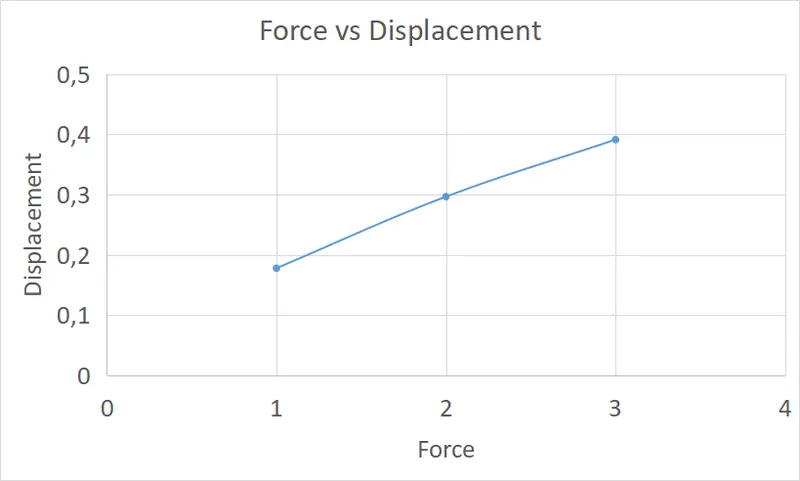
Step i	ΔFi	ui	Δui	F(ext)i	f(int)i	R
1	1.0	0.1777	0.1777	1	1.0005	0.0005
2	1.0	0.2965	0.1371	2	2.0032	0.0032
3	1.0	0.3912	0.1041	3	3.0019	0.0019

Exact values:

The values are calculated using scientific calculator.

• Take, F(u) = u³+9u²+4u = 1
  • u = 0.1776
• Take, F(u) = u³+9u²+4u = 2
  • u = 0.2962
• Take, F(u) = u³+9u²+4u = 3
  • u = 0.3910

Comparison:

F(ext)i	Explicit	Implicit	Exact
1	0.25	0.1777	0.1776
2	0.3651	0.2965	0.2962
3	0.4562	0.3912	0.3910

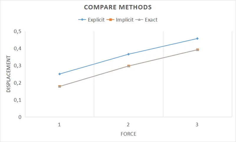
The implicit and exact methods give nearly same results. While the explicit method results are away from the results using exact method.

Conclusion:

The given equation has been solved for explicit and implicit numerical analysis methods. And then, the methods are compared and plotted as a graph.