Week - 2 - Explicit and Implicit Analysis

Week - 2 - Explicit and Implicit Analysis

A Differential equation can be solved by using either Explicit or Implicit Analysis by integrating with time using time step intervals.

They are best suited to be used for solving dynamic problems.

Explicit Analysis:

In Explicit analysis, equilibrium doen't need to converge in every time step. It assumes that the equilibrium exists at every time step, but for the explicit analysis the time step is calculated automatically by the solver based on the material properties like density, young's modulus and the length of the samllest element.

Implicit Analysis:

In Implicit analysis, equilibrium needed to be converged in each time step/increament. So the time taken for solving using implicit increases as the convergence is necessary at every time step.

The advantage is the time step can be high and so the overall time is decreased.

The choice of the analysis type depends on the overall time interval,

If the simulation is to be completed in several seconds, explicit analysis take too much time to complete the simulation as the time step is very small. So, implicit analysis is optimal as the time step can be given manually.

If the simulation is to be completed in fraction of seconds, explicit analysis is better suited as it can be completed in very less time.

AIM: Solve the given equation F(u) = `u^3+9u^2+4u` using both Explicit and Implicit Methods for a simple bar unber tension.

Calculations:

For the equation given, stiffness k(u) = `(df)/(du) = 3u^2 +18u+4`

f(u) is internal force and u is displacement

Explicit Analysis:

Here we use load control scheme to plot external force vs displacement curve, where three external equal load increaments are taken. (`DeltaF = 1`)

Taking intially `u_0` = 0.0

substituting u in f(u) gives the internal force developed for the displacement we got due to `DeltaF` applied

F(u) is the cummulative force applied externally after time step

Using `DeltaF = kDeltau` and `u_i = u_(i-1)+Deltau_i` we get value of `Deltau` and subsequent u for the next time step.

	u	f(u) Internal	F(u) external	DeltaF	k(u)	Deltau	Residual R = f(u) - F(u)
u0	0	0	0	1	4	0.25	0
u1	0.25	1.578125	1	1	8.6875	0.115108	0.578125
u2	0.365108	2.708836	2	1	10.97185	0.091142	0.708836
u3	0.45625	3.793454	3				0.795434

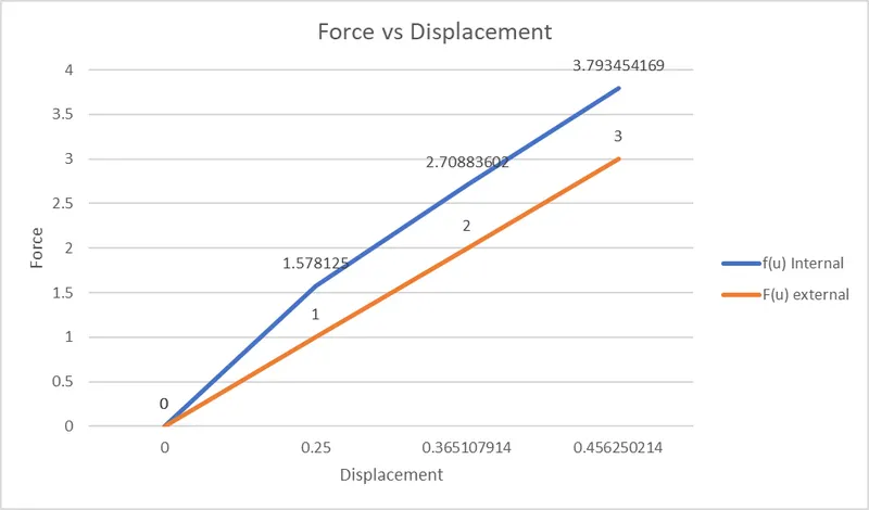
We can See that internal forces and the applied external forces doesn't converge

Internal force vs displacement graph

Implicit Analysis:

Here we use Newton-Raphson method is used at the end of each step to enforce equilibrium before next step

This equilibrium is maintained when stiffness is linear for every time step

For the equation given, stiffness k(u) = `(df)/(du) = 3u^2 +18u+4` which is non-linear

R = f(u)_internal - F(u)_external; `(df)/(du) = k(u)`

So, adjustment is made to displacement, by minimizing the residual by expanding the residual with Taylor series expansion and neglecting the higher order terms.

`deltau_(i+1) = -R_i/(k(u_i))`

where `(R_i)` is the residual at the end of `i^th` time step

These adjustment to displacement and iterations are done till R reaches the given tolerance value of 0.001

Taking `u_0` = 0 intially

Similar to explicit analysis. u, k(u) and `Delta u` is found and correction u is found from above equation

When R reaches tolerance value the u and `Deltau` is finalized for that step and is taken in next step for displacement.

		f(u) Internal	F(u) external	`DeltaF`	k(u)	`Deltau`	R	R check	Iteration 1	u correction `u_i`
`u_0`	0.000	0.000	0.000	1.000	4.000	0.250	0.000	< 0.001	No iterations required
`u_1`	0.250	1.578	1.000	1.000	8.688	0.115	0.578	> 0.001	iterations required	-0.06655
`u_1^1`	0.183	1.043	1.000	1.000	7.403	0.135	0.043	> 0.001	iterations required	-0.00579
`u_1^2`	0.178	1.000	1.000	1.000	7.293	0.137	0.000	<0.001	No iterations required
`u_2`	0.315	2.182	2.000	1.000	9.963	0.100	0.182	> 0.001	iterations required	-0.01828
`u_2^1`	0.297	2.003	2.000	1.000	9.601	0.104	0.003	> 0.001	iterations required	-0.00035
`u_2^2`	0.296	2.000	2.000	1.000	9.594	0.104	0.000	< 0.001	No iterations required
`u_3`	0.400	3.109	3.000	1.000	11.688	0.086	0.109	> 0.001	iterations required	-0.00929
`u_3^1`	0.391	3.001	3.000	1.000	11.499	0.087	0.001	= 0.001	No iterations required

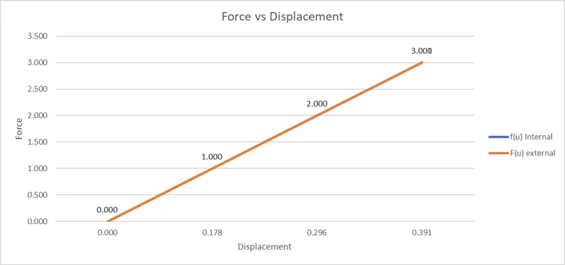
We can see that internal forces and exteranl forces are in equlibrium after corrections are made to displaccement and iterations are more for every time step.

Force vs Displacement Graph

.

Conclusion:

We can observe that the plot of explicit analysis deviates from exact solution due to large residuals, steps, and equlibrium is assumed. This is converged when smaller time step is used.

We can observe that the plot of implicit analysis corrects to exact solution due to application of Newton-Raphson method to adjust the displacement and equlibrium is enforced.

The given equation F(u) = u3+9u2+4u is solved using both implicit and explicit analysis.