Week - 2 - Explicit and Implicit Analysis

' Aim:
The Aim of this Challenge is to Study the Two diffent Methods to solve the General Equation of Structural Analysis.

Description:

The Two different Methods to Solve the General Equation of Motion are Explicit and Implicit Methods. Both Equations aims to solve the Governing Equation as shown below.

`[M]{ddotx}+[C]{dotx}+[k]{x}=f(t)`

Where [M] is the Inertial mass Matrix

[C] is the Damping Matrix

[K] is the stiffness Matrix

f(t) = External Force.

`{ddotx}` = Acceleration Vector.

`{dotx}`= Velocity Vector.

`{x}` = Displacement Vector.

The Implicit & Explicit methods are generally used to solve the Dynamic Problems, which includes the inertial & Damping effects. The General Rule of Thumb is that if the Frequency of External Excitation force is greater than 1/3rd of the First Natural Frequency, then we cannot ignore the inertial effects of the system and the system has to be considered as dynamic system. On other case if the Frequency of the External Excitation force is very less than the 1/3rd of the First natural frequency, we will consider the system to be static and the system can be analysed using the conventional static solver. The Implicit & Explicit solvers can be used to solve the static Problems, but it is computationally expensive.

Hence inorder to solve the Dynamic Problems Implicit & Explicit methods are used in Dynamic Solvers. Ls-Dyna is one solver which is intended for analysing Dynamic Problems.

Explicit Method:

The Meaning of Word Explicit means "stated Clearly". If you can Rewrite a mathematical equation with knowns on one side and unknowns on other side it is called as "Explicit Equation". In Explicit Method the solution at next step is found from the known values in the Previous step. Generally the Dynamic Equations are time dependant and hence we can say that the solution at next time step is found from slope values of present time step in Dynamic Method.

The Equation given for solving with Explicit Analysis is `F(u) = u3+9u2+4u.` Here the Force is the function of displacement. The Slope (Derviative) of this Equation reporesents the Stiffness of the system.

`F(u) = u^3+9u^2+4u`, Whereas its derviative (Slope) is given by `3u^2+18u+4`. Assuming the Increment of `DeltaF`=1.In this Explicit Analysis we will assume that we didn't know the Excat relation between the Force and Displacement and we will know only the stiffness relation with Displacement. Hence the Force is incremented step by step, and for Each Step the Incremental Displacement is found out from the relation`DeltaF=K*DeltaU`. The Calculated Incremental Displacement is added to the Previous displacement to find out the Displacement at the Next Step. For Example in first Increment. The Displacement is set as 0. Since the Force is the Function of Displacement the Real force also becomes Zero. similarly the Stiffness of the system at u=0 comes out to be 4. From the relation `DeltaF = K* DeltaU`, & We fixed the `Delta F` the `DeltaU`Calculated to be 0.25. Which is added to the Initial Displacement value of 0 gives the Displacement for next Increment as 0+0.25 = 0.25. The Difference between the Real Force(Force calculated from known Force Displacement Relationship) and the Incremental Force is called as "Error" or "Residue"The Equation is solved Explicitly and the Results are given below`

Increments	Displacement Calculated	Excat Force	Stiffness	Residual	Force increments
1	0	0	4	0	0
2	0.25	1.578125	8.6875	0.578125	1
3	0.365108	2.7088	10.97186	0.708837	2
4	0.45625	3.7934	12.83699	0.793451	3
5	0.53415	4.8568	14.47065	0.8568	4
6	0.603255	5.907804	15.95034	0.907904	5
7	0.66595	6.950546	17.31757	0.950546	6
8	0.723695	7.987414	18.59771	0.987414	7
9	0.777465	9.019867	19.80773	1.01	8
10	0.82795	10.04887	20.9596	1.0488	9

The graph is drawn for excat Force Displacement Relation and Calculated Force Displacement Relation is given below. The Calculated Force Displacement Curve has similar Slope Compared with Excat Force Displacement Relation. But we can clearly the values are different.

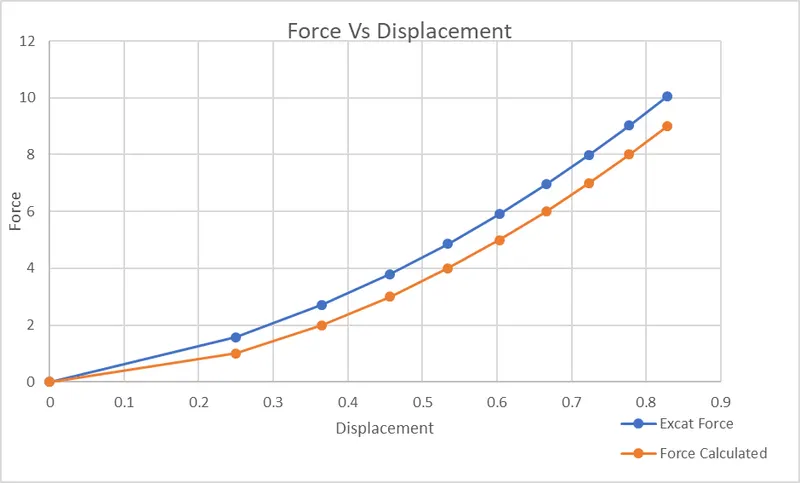
The Equation is again solved by same Procedure described above but this time with the `DeltaF=0.5`, for same 10 Increments and the Results are Given below. You can see for Each Increment, the Residual Value is very Less compared to Previous Table.

S.NO	Displacement Calculated	ExcatForce	Stiffness	Residual	Force increments
1	0	0	4	0	0
2	0.125	0.642578	6.296875	0.1425	0.5
3	0.204404	1.202185	7.8046	0.202185	1
4	0.268469	1.741907	9.0486612	0.241907	1.5
5	0.323726	2.272	10.14	0.272017	2
6	0.373029	2.796379	11.1312	0.2963	2.5
7	0.417945	3.316888	12.047	0.3168	3
8	0.459449	3.834623	12.9033	0.334623	3.5
9	0.498199	4.3507	13.7122	0.35027	4
10	0.534633	4.863839	14.48089	0.363839	4.5

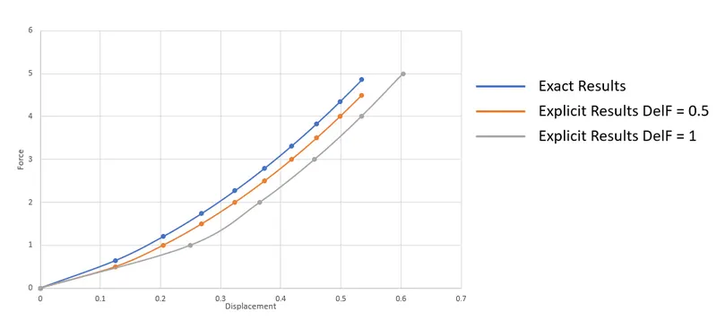
It is Clear from the Below graph that the Explicit Method gives better results when the Incremental Value `DeltaF`is small`

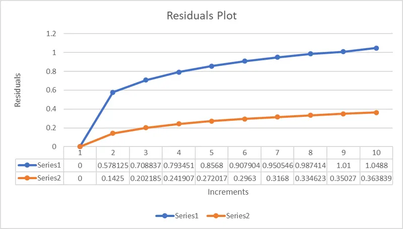
The Residual Plot for `DeltaF=1`& `DeltaF=0.5`is given below and it is clear that `DeltaF=0.5`has lower Residuals. Here the Blue Line indicates the Residuals for DeltaF=1 and Orange Line indicates the DeltaF=0.5

Implicit Method:

The Implicit Analysis is same as Explicit Analysis, but at end of Each Step, the Newton_Raphson method is used to enforce the Equillibrium. since the Force & Displacement is Related by the Equation `DeltaF = K* Deltau`where K is the Function of Displacement, the Corrections must be done to Displacement term to enforce Equillibrium between the External & Internal Forces. The Equillibrium will not be acheived until we calculate the particular Displacement above which Displacement will nolonger be a linear Function. Inorder to find the Corrected Displacement we use the Correction factor obrained from Newton_Raphson Iterations for minimization of Residuals`

The Same Equation`F(u) = u3+9u2+4u.` is solved by Implicit Method, The Results are indicated in the Table Below.

Implicit Method Calculation:

`uo =0, K(0)=4, DeltaF=1; Deltau =(DeltaF)/K = 0.25`

`u(0.25)=1.578125`

Residual `R(0.25)= 0.578125: K(0.25)=8.6875`

`delu1 = -(8.6875)^-1 *(0.578125) = -0.06654` _ (Correction of Deltau using Newton_raphson Correction Factor)

`Deltau1 = 0.25-0.06654 = 0.18346 (new Incremental Displacement`

F(0.18346) = 1.042933

Updated Residual R(0.18346) = 0.042933>0.001, Hence Displacement need to be corrected again.

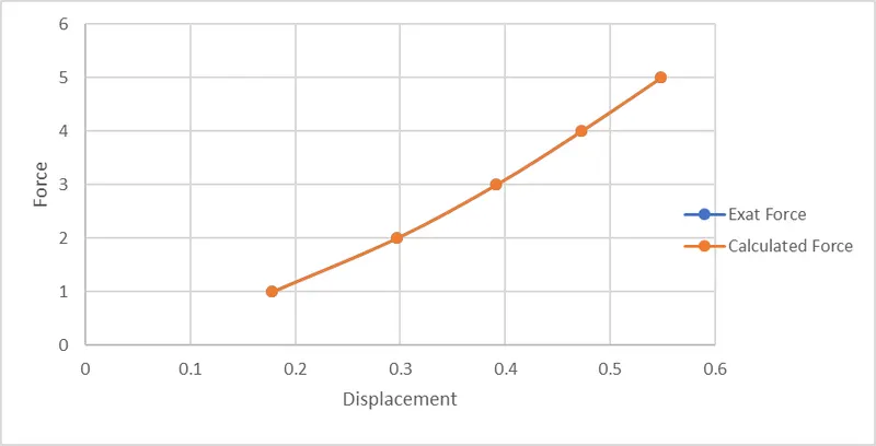
You can se that the Residuals obtained when Using the Implicit Method is Very Low. The Results obtained from Implicit Analysis is much more accurate than results obtained from Explicit Analysis.

S.No	Displacement	Exat Force	Calculated Force	Residuals
1	0.17776	1	1.000315	0.000315
2	0.2963	2	2.001356	0.001356
3	0.3911	3	3.000855	0.000855
4	0.47215	4	4.000185	0.000185
5	0.5481	5	5.00012	0.00012

Observations:

• Explicit Analysis is dependant on the Incremental Value of Force to obtain the Excat Solution. The Residual obtained `DeltaF=0.5`is much smaller than the Residuals obtained when `DeltaF=1`.
• The Explicit Analysis Tend to Deviate from the Real Solution for Each and Every Increment. we can infer this from the Residual Vs Increment Plot of Implicit Analysis.
• Implicit Analysis uses the Minimization of Residuals to Correct the Displacement. Hence the Residuals obtained in Implicit Analysis is Very Low.
• Implicit Analysis doesn't depend incremental Value of DeltaF to obtain more excat solution.
• When Considering the Problem under study, Implicit method is better in obtaining the Excat Solutions, but when Considering the Time of Computation Explicit method solves the problem relatively more faster than implicit method for every Incremental Force.
• But Generally, Explicit Dynamic analysis is performed by solving inversion of Mass-matrix and Implicit Dynamic analysis is performed by solving the inversion of Stiffness matrix.
• The Inversion of Mass Matrix during Dynamic Analysis is very Computationally Economical when compared to Inversion of Stiffness Matrix.
• Hence regarding Computational time, Explicit Scheme solves the Problem much faster when compared to Implicit Scheme.
• The Explicit Dynamic analysis is conditionally stable, which means the incremental timestep has to be less than (Characteristic Length/Speed of Sound in material).
• The Implicit Dynamic Analysis is unconditionally stable. Hence it can solve for any larger timestep.

Conclusion:

The Explicit and implicit method of solving the Dynamic Structural Problems is understood.