Week - 2 - Explicit and Implicit Analysis

Week - 2 - Explicit and Implicit Analysis

Aim : To solve the equation `F(u) = u^3+9u^2+4u` in Explicit and implicit methods with tolerance of 0.001.

Theory :

Difference between Implicit and Explicit methods :

IMPLICIT	EXPLICIT
It deals static and dynamic problems	It deals dynamic and shock problems
it is always stable	It is conditional stability
It is global resolution i.e need of convergence	It is element by element calculation
It is too expensive	It is less expensive
Time step is very large	Time step is very low
Low robustness	High robustness

Implicit Time Integration :

Advantages :

• It is Unconditionally stable(no timestep limit).
• Used in static analysis.
• It is relatively inexpensive for long duration analysis.

Disadvantages :

• Often requires a large amount of memory.
• It can cause problems with strongly non-linear models.

Explicit Time Integration :

Advantages :

• Computationally fast.
• Low core / RAM intensive.

Disadvantages :

• Conditionally stable(timestep limit).
• Expensive to conduct long duration analysis.

Applications :

Implicit :

• Linear and non-linear static analysis.
• Low rate dynamic analysis.
• Vibration and Modal analysis.
• Strength and buckling.
• Springback.
• Gravity loading and pre-loading.

Explicit :

• High rate dynamic analysis.
• Impact / penetration problems.
• Car crash.
• Explosives.

The Problem

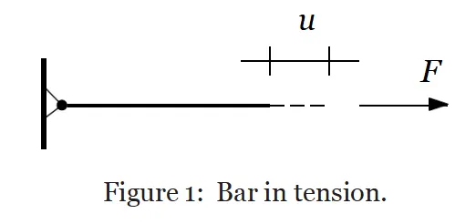
Consider the case of a simple bar in tension as shown in Figure 1. Suppose that the force in the bar is a nonlinear function of the displacement.

`F(u) = u^3+9u^2+4u` ( 1 )

From ( 1 ) it follows that the stiffness of the bar is

`K(u) = (dF)/(du) = 3u^2+18u+4` ( 2 )

Explicit Analysis :

If nonlinear force versus displacement relationship is not known, but the stiffness is known, it is possible to construct the graph of force versus displacement numerically. One method is to use an incremental explicit load control scheme. This is illustrated next. For this example three equal load increments (or steps) of ∆F = 1 unit each are used to load the tension bar. The variables used are u for displacement, f for internal force in the bar, F for external force applied to the bar and k for stiffness.

Incremental displacements or incremental externally applied forces are represented as ∆u or ∆F , respectively. Use is made of the relationship ∆F = k∆u. The analysis proceeds as follows :

Step 1

`u_{0}=0.0, ⇒k(u_{0})=4, ΔF=1, Δu_{1}=(ΔF)/(k(u_{0}))=0.25, u_{1}=u_{0}+Δu_{1}=0.25`

Step 2

`u_{1}=0.25, ⇒k(u_{1})=8.688, ΔF=1, Δu_{2}=(ΔF)/(k(u_{1}))=0.1151, u_{2}=u_{1}+Δu_{2}=0.3651`

Step 3

`u_{2}=0.3651, ⇒k(u_{2})=10.9717, ΔF=1, Δu_{3}=(ΔF)/(k(u_{2}))=0.0911, u_{3}=u_{2}+Δu_{3}=0.4562`

Finally, from the three steps the following results are obtained.

`F _{e x t e r n a l} = Δ F + Δ F + Δ F = 3`

`f_{Int}= u_{3}^3 + 9 u_{3}^ 2 + 4 u_{3} = 3.7928`

Table :

Step i	`DeltaF_{i}`	`Deltau_{i}`	`u_{i}`	`(F_{ext})_{i}`	`(f_{Int})_{i}`	`R = f_{Int}-F_{ext}`
1.0	1.0	0.2500	0.2500	1.0	1.5781	0.5781
2.0	1.0	0.1151	0.3651	2.0	2.7080	0.7080
3.0	1.0	0.0911	0.4562	3.0	3.7928	0.7928

Implicit Analysis :

• Implicit analysis is similar to explicit analysis, except that at the end of each step, Newton-Raphson iterations are introduced to enforce equilibrium before moving to next step. Basically, incremental force is applied to advance the solution forward at the beginning of a step. Anyway, internal forces and external forces will not be in equilibrium unless the stiffness is linear for the given step.
• Therefore, in order to achieve equilibrium, corrections should be made to the displacement.
• This is acquired by using Newton-Raphson iterations to reduce the residual, `R=F_{Internal}−F_{external}`
• Expanding the residual as a Taylor series about the current displacement `u^j` gives

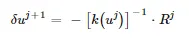
• By neglecting higher order terms in above series, i.e. `R^(j+1)=0` and solving for `δu^(j+1)` the following correction can be obtained

• The iteration variable here is j and it may take several iterations for the norm of the residual, R to be reduced below the chosen tolerance criteria 0.01.
• The implicit analysis proceeds as follows ;

Step 1

`u_{0}=0.0, ⇒k(u_{0})=4, ΔF=1, Δu_{1}=(ΔF)/(k(u_{0}))=0.25, u_{1}=u_{0}+Δu_{1}=0.25`

Checking the residual,

`F_{external} =Delta F=1`

`f_{Internal}= u_{1}^3 + 9 u_{1}^ 2 + 4 u_{1} = 1.578`

`R^((0))= f_{Internal}-F_{external}=0.578`

`R ^( (0) ) > 10 ^(− 2) ⇒ ` Newton-Raphson iterations are necessary.

Calculate the correction to `u_{1} = u_{1}^((0))`

`δ u ^(( 1) ) = − [ k ( u_{1} ^(( 0) ) ) ] ^(− 1) ⋅ R ^(( 0 )) = − ( 8.6875 )^(− 1) ⋅ 0.578 = − 0.0665`

The updated value of `u _{1} ^(( 1) ) = u_{1}^(( 0) ) + δ u ^(( 1) ) = 0.25 − 0.0665 = 0.1835`

Checking the residual again,

`F_{external} =Delta F=1`

`f_{Internal}= (u_{1}^((1)))^3 + 9 (u_{1}^((1)))^ 2 + 4 u_{1}^((1)) = 1.0432`

`R^((1))= f_{Internal}-F_{external}=0.0432`

`R ^( (1) ) > 10 ^(− 2) ⇒ ` Newton-Raphson iterations are necessary.

Calculate the new total correction to `u_{1} = u_{1}^((0))`

`δ u ^(( 2)) = δ u ^(( 1))− [ k ( u ^(( 1))) ] ^(− 1) ⋅ R ^(( 1 )) =− 0.0665− (7.404 )^(− 1) ⋅ 0.0432 = − 0.0723`

The updated value of `u _{1} ^(( 2) ) = u_{1}^(( 0) ) + δ u ^(( 2) ) = 0.25 − 0.0723 = 0.1777`

Checking the residual again,

`F_{external} =Delta F=1`

`f_{Internal}= (u_{1}^((2)))^3 + 9 (u_{1}^((2)))^ 2 + 4 u_{1}^((2)) = 1.0006`

`R^((2))= f_{Internal}-F_{external}=0.0006`

`R ^( (2) ) > 10 ^(− 2) ⇒ ` Newton-Raphson iterations are not necessary.

Therefore, the final value is `u_{1} = u_{1}^((2)) = 0.1777`

Step 2

`u_{1}=0.1777, ⇒k(u_{1})=7.2933, ΔF=1, Δu_{2}=(ΔF)/(k(u_{1}))=0.1371, u_{2}=u_{1}+Δu_{2}=0.3148`

Checking the residual,

`F_{external} =Delta F+Delta F=2`

`f_{Internal}= u_{2}^3 + 9 u_{2}^ 2 + 4 u_{2} = 2.1822`

`R^((0))= f_{Internal}-F_{external}=0.1822`

`R ^( (0) ) > 10 ^(− 2) ⇒ ` Newton-Raphson iterations are necessary.

Calculate the correction to `u_{2} = u_{2}^((0))`

`δ u ^(( 1) ) = − [ k ( u_{2} ^(( 0) ) ) ] ^(− 1) ⋅ R ^(( 0 )) = − ( 9.9637 )^(− 1) ⋅ 0.1822 = − 0.0182`

The updated value of `u _{2} ^(( 1) ) = u_{2}^(( 0) ) + δ u ^(( 1) ) = 0.3148 − 0.0182 = 0.2966`

Checking the residual again,

`F_{external} =Delta F+Delta F=2`

`f_{Internal}= (u_{2}^((1)))^3 + 9 (u_{2}^((1)))^ 2 + 4 u_{2}^((1)) = 2.0042`

`R^((1))= f_{Internal}-F_{external}=0.0042`

`R ^( (1) ) < 10 ^(− 2) ⇒ ` Newton-Raphson iterations are not necessary.

Therefore, the final value is `u_{2} = u_{2}^((1)) = 0.2966`

Step 3

`u_{2}=0.2966, ⇒k(u_{2})=9.6027, ΔF=1, Δu_{3}=(ΔF)/(k(u_{2}))=0.1041, u_{3}=u_{2}+Δu_{3}=0.4007`

Checking the residual,

`F_{external} =Delta F+Delta F+Delta F=3`

`f_{Internal}= u_{3}^3 + 9 u_{3}^ 2 + 4 u_{3} = 3.1121`

`R^((0))= f_{Internal}-F_{external}=0.1121`

`R ^( (0) ) > 10 ^(− 2) ⇒ ` Newton-Raphson iterations are necessary.

Calculate the correction to `u_{3} = u_{3}^((0))`

`δ u ^(( 1) ) = − [ k ( u_{3} ^(( 0) ) ) ] ^(− 1) ⋅ R ^(( 0 )) = − ( 11.6942 )^(− 1) ⋅ 0.1121 = − 0.00958`

The updated value of `u _{3} ^(( 1) ) = u_{3}^(( 0) ) + δ u ^(( 1) ) = 0.4007 − 0.00958 = 0.3911`

Checking the residual again,

`F_{external} =Delta F+Delta F+Delta F=3`

`f_{Internal}= (u_{3}^((1)))^3 + 9 (u_{3}^((1)))^ 2 + 4 u_{3}^((1)) = 3.0008`

`R^((1))= f_{Internal}-F_{external}=0.0008`

`R ^( (1) ) < 10 ^(− 2) ⇒ ` Newton-Raphson iterations are not necessary.

Therefore, the final value is `u_{3} = u_{3}^((1)) = 0.3911`

Table :

Step i	`DeltaF_{i}`	`u_{i}`	`(F_{ext})_{i}`	`(f_{Int})_{i}`	`R = f_{Int}-F_{ext}`
1.0	1.0	0.1777	1.0	1.0006	0.0006
2.0	1.0	0.2966	2.0	2.0042	0.0042
3.0	1.0	0.3911	3.0	3.0008	0.0008

Graph :

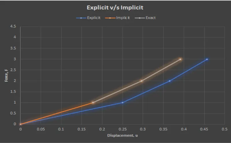
• We can clearly see that Explicit curve drifts from the exact solution, this is due to lack of equilibrium between internal and external forces.
• Whereas Implicit curve comes close to the exact curve.Here, Newton-Raphson iterations correct the incremental steps so that the solution comes close to exact curve, according to the specified tolerance. Excellence is achieved within 3 increments and in each step only 2 Newton-Raphson iterations are required.

Conclusion :

Thus the given equation is solved in both implicit and Explicit methods. From the above observations we can say that implicit method wil give better results in non linear static problems when time and computational cost are considered.