Week - 2 - Explicit and Implicit Analysis

Solution of a simple structural problem using explicit and implicit methods

1. Explicit versus Implicit schemes

All the Finite element methods solve the differential equations using numerical methods. These numerical methods can be explicit or implicit based on the requirements and problem. For example, take a general problem described by equation `(d vec u)/dt= F(vec u)`; This means the force is a function of displacement 'u' and we want to solve for 'u'. Since its a transient simulation we are interested in outcomes at time t, t+1, ......, t+n. `

Let us denote time by 'n'. So (n) to (n+1) is one-time step and for explicit method; `u(n+1)=u(n)+Delta t*F(u(n))` where the L.H.S denote the displacement at (n+1)th time step and R.H.S. means the sum of displacement at n and displacement due to force at nth time step. In other words, in the explicit method, all the terms from the previous time step are used to approximating the outcome for the next time step.  

On the other hand, for implicit analysis using the same notations; `u(n+1) = u(n)+ Delta t * F(u(n+1))`i.e. the displacement at the (n+1)th time step is expressed as previous displacement plus force-displacement as a function of (n+1)th displacement instead of (n)th displacement terms. This creates the need to use matrix inversion for solving the equations. The complete method becomes:

`u(n+1) = u (n) + Delta t * F(u(n+1))`

`implies (I-A)* Delta t *u(n+1) = u(n)`; Here I denotes one identity matrix that is defined to solve the equation and using the matrix inversion the u(n+1) is defined. 

For example; To solve `M* (d^2u)/dt^2+ ku= F(t)`-----(1)

At t=0 we know the values of displacement 'u' and velocity 'v' which can be used to calculate [M] and [k] which are mass and stiffness matrices. These values are then used to find out the acceleration which further provides velocity and displacement. 

The above equation (1) can be written as ; `{a}= [M]^-1({F(t)}-[k]{u})`

Further, velocity and displacements can be calculated as: 

`v* Delta t= v(0) +a Delta t`

`u(Delta t)= u(0)+v(0)*Delta t + 1/2 a Delta t^2`

For the implicit method, we compute [M] and [k] not at t=0 but at `Delta t` and use the method as explained above. So, it requires more calculations and the cost of computing becomes large. `

2. Calculation of results for a Simple bar under tensile loading.

consider the below-given figure which shows a bar constrained at one end and loaded at the other end with a force which is given as a function of displacement 'u'.

 

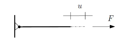
The internal resisting force is defined as `f(u)= u^3+9u^2+4u` -------------(1)

We are going to use explicit and implicit schemes one by one to find out the displacements and values of forces. The tolerance value is given to be 0.001.

2.1 Explicit scheme:

hooke's Law `F= k*u`is used to express `k(u)= (df)/(du)`where k(u) represents stiffness as a function of displacement u.

This leads to `k(u)= 3*u^2+18u+4` ------------(2)

Then the incremental explicit load control scheme is used with step of `Delta F=1` is used to load the bar. Three such load steps will be calculated to get the values. The incremental displacement is represented as `Delta u`. The relation `Delta F= k Delta u` is used to get the incremental displacement as `Delta u = (Delta F)/(k(u))`  --------(3)

Step 1

We have initially,`Delta F=1` ,   `u(0) = 0`   so using equation (2) we get `k(u)= 3*u^2+18u+4``implies k(u0) =4` and using equation (3) we get `Delta u1= 1/4`

So, `u1= u0+Delta u1`  `implies u1= 1/4`.

Step 2

at `u1= 1/4`  we get `k(u1)= 8.6875` using eq. (2) and again `Delta F=1` leads to `Delta u2= (DeltaF)/(k(u1))` `implies Delta u1= 1/8.6875`   So for this step `u2 = u1+Delta u2``implies u2= 0.36511`

Step 3

at `u2=0.36511`  we get `k(u2)= 10.97190`  using eq. (2) and `Delta u3= (Delta F)/(k(u2))`  `implies Delta u3= 1/10.9719` .

So at the end of step 3 we get `u3= u2+Delta u3 implies u3= 0.45625`

Further,  Excel was used to perform more steps using the formulae as discussed above. Also, the value of internal force at the end of each step was calculated using equation (1) and the external force was computed using `F= sumDelta F`  and residual value defined as `R = f-F` where f is internal force and F represents the externally applied force.

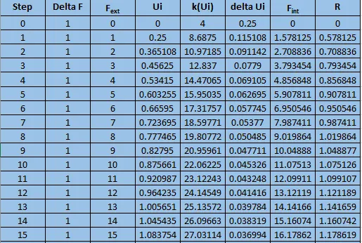
Fig 2.1: The calculation of values using the explicit scheme.

A plot of the residual value gives an idea that initially, the residual was increasing sharply but after some iterations, the slope changed and it would come below the tolerance of 0.001 after many more iterations.

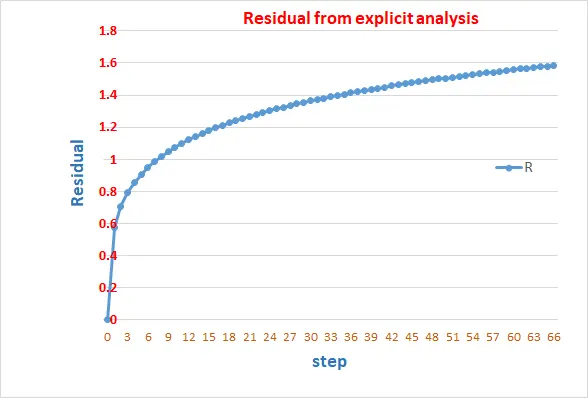
Fig 2.2: The plot of residual

A comparison of the value for external force and internal force was made. As it was a static structural problem, both the forces are expected to be in equilibrium hence they should be equal. 

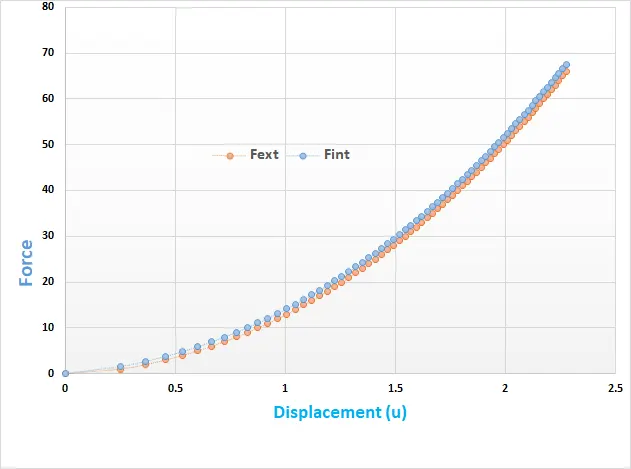
Fig 2.2: Comparison between the external and internal force values with respect to displacement

as clear from the above graph the calculated values deviate from the actual values and this fact can be accepted as a drawback of the explicit scheme. Moreover, each time step in the Explicit scheme is very fast but the method is stable only when the time step is very small. Courant's condition dictates that the timestep must be smaller than an elastic wave to propagate from one side of the element to the other side. 

Since there is a condition for the method to be stable, it is called to be a conditionally stable method.

2.2 Implicit Scheme

An implicit analysis is the same as explicit analysis except that at the end of each step, Newton-Raphson iterations are used to enforce equilibrium before moving to the next step. Basically, an incremental force is applied to advance the solution forward at the beginning of a step. However, internal forces and external forces will not be in equilibrium unless stiffness is linear for the given step. Hence, in order to achieve equilibrium, corrections must be made at the end of each step. This is done using the Newton- Raphson method to minimise the residual `R(u)= f-F`

In practical applications, a tolerance value is chosen which is used to state that the forces are in equilibrium, ignoring the error below it. A derivation of the residual using Taylor series expansion yields a correction to the value of u as `delta u(j+1)= -[k(u(j))]^-1*R(j)`  where j denotes the iteration number and it may take several iterations for the `normR` to fall below the set tolerance. For our case, the tolerance is 0.001.

Step 1

We have initially,`Delta F=1` ,   `u(0) = 0`   so using equation (2) we get `k(u)= 3*u^2+18u+4``implies k(u0) =4` and using equation (3) we get `Delta u1= 1/4`

So, `u1= u0+Delta u1`  `implies u1= 1/4`.

next, check the residual for `Delta F=1`, using Eq. (1) we get the `f = u^3 + 9u^2+4u implies f= 1.578125` and we have `F= sum Delta F implies F= 1` So, residual `R(0)= f1-F1 = 1.578125-1 implies R(0)= 0.578125` which is more than tolerance value 0.001 hence , Newto -Raphson iterations are needed.  

Calculate the correction to  `u1=u1(0)`.   We have `delta u(1)= [-k(u1)]^-1*R(0) and k(u1)= 3*0.25^2+18*0.25+4 = 8.6875 implies delta u(1)= -0.66547`

So the updated value of u(1) becomes `u1 = u1+ delta u(1) implies u(1)= 0.183453`  

Again checking the residual, we get;

`f= f(u1-updated) implies f = 1.042881`  So Residual comes out to be `1.042881-1=0.042881 ` which is more than 0.001. So, again correction is needed. We need to calculate the new total correction to the u(1) given by `delta (u2) = delta (u1) - [k(u1)]^-1*R(1)`  We have `[k(u1)]^-1 = [3* 0.183453^2+ 18*0.183453+4 ]^-1 = 0.135078`

This give the correction `delta (u2)= -0.072339` and the update value of u becomes `u1+ deltau (2) implies u(1) = 0.177661` putting this value of u into Eq. (1) gives `f = 1.000322` and the residual becomes 0.000322 which is less than our tolerance 0.001. 

So at the end of step 1 we get u(1) = 0.177661 and f= 1.000322.

Step 2

`Delta F=1` ,   `u(1) = 0.177661`   so using equation (2) we get `k(u)= 3*u^2+18u+4``implies k(u1) =7.292588` and using equation (3) we get `Delta u2= 1/7.292588 = 0.137125`

So, `u2= u1+Delta u2`  `implies u2= 0.314786`.

next, check the residual for `Delta F=1`, using Eq. (1) we get the `f = u^3 + 9u^2+4u implies f= 2.182148` and we have `F= sum Delta F implies F= 1+1=2` So, residual `R(0)= f1-F1 = 2.182148-2 implies R(0)= 0.182148` which is more than tolerance value 0.001 hence , Newton -Raphson iterations are needed.  

Calculate the correction to  `u2=u2(0)`.   We have `delta u(1)= [-k(u1)]^-1*R(0) and k(u1)= 3*0.314786^2+18*0.314786+4 implies delta u(1)= -0.018282`

So the updated value of u(2) becomes `u2 = u2+ delta u(1) implies u(1)= 0.296504` 

Again checking the residual, we get;

`f= f(u2-updated) implies f = 2.003315`  So Residual comes out to be `2.003315-2=0.003315 ` which is more than 0.001. So, again correction is needed. We need to calculate the new total correction to the u(2) given by `delta (u2) = delta (u1) - [k(u2)]^-1*R(2)`  We have `[k(u2)]^-1 = [3* 0.296504^2+ 18*0.296504+4 ]^-1 `

This give the correction `delta (u2)= -0.018627` and the update value of u becomes `u2+ deltau (2) implies u(2) = 0.296159` putting this value of u into Eq. (1) gives `f = 2.000000353` and the residual becomes 0.000000353 which is less than our tolerance 0.001. 

So at the end of step 2 we get u(2) = 0.296159 and f= 2.000000353

Step 3

`Delta F=1` ,   `u(2) = 0.296159`   so using equation (2) we get `k(u)= 3*u^2+18u+4``implies k(u2) =9.593992` and using equation (3) we get `Delta u3= 1/9.593992 = 0.104232`

So, `u3= u2+Delta u3`  `implies u3= 0.400391`.

next, check the residual for `Delta F=1`, using Eq. (1) we get the `f = u^3 + 9u^2+4u implies f= 3.108568` and we have `F= sum Delta F implies F= 1+1+1=3` So, residual `R(0)= f3-F3 = 3.108568-3 implies R(0)= 0.108568` which is more than tolerance value 0.001 hence , Newton -Raphson iterations are needed.  

Calculate the correction to  `u3=u3(0)`.   We have `delta u(1)= [-k(u3)]^-1*R(0) and k(u3)= 3*0.400391^2+18*0.400391+4 implies delta u(3)= -0.009289`

So the updated value of u(3) becomes `u3 = u3+ delta u(1) implies u(3)= 0.391102` 

Again checking the residual, we get;

`f= f(u3-updated) implies f = 3.00087823`  So Residual comes out to be `0.000878 ` which is less than 0.001 and this means no further corrections are needed. 

At the end of step 3, we get u3= 0.391102 and f= 3.00087823.

 The data was tabulated in Excel and a comparison between the two force values was made as shown in the below figures.

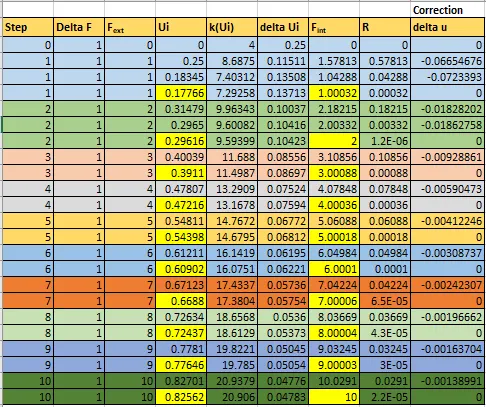
Fig 2.2.1: The table used to calculate values up to 10 steps

As clear from the above table, the residuals fall quickly with the use of implicit scheme and error is very less as compared to the explicit scheme. Also at the end of 10 the step, the exact value was obtained.

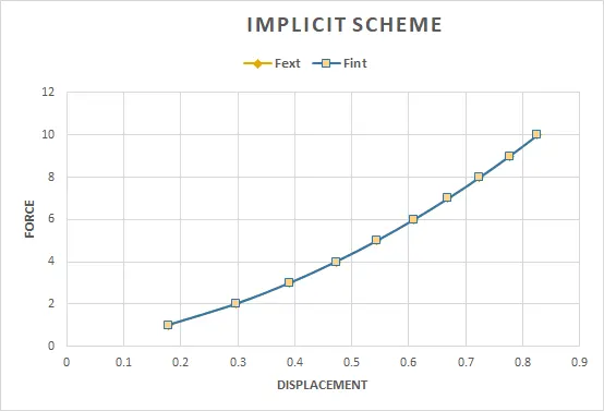
Fig 2.2.2: the comparison of actual and calculated data using the implicit scheme

Note: As clear from the above plot, the results match the real values more closely as compared to the explicit scheme.

3. Conclusion

A comparison of the output obtained using the explicit and implicit scheme is shown in the below-attached plot where Fext refers to the actual value.

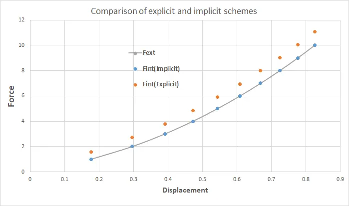
Fig 3.1: The comparison of explicit and implicit schemes.

The above plot can be used to conclude that results from the explicit scheme deviate significantly while the outcomes of the implicit scheme adhere to the exact value more accurately. However, the implicit scheme is much complex and needs more computation than the explicit scheme. This may lead to increase in simulation cost when using the implicit scheme for complex models which is one of its major drawbacks. 

On the other hand, the explicit scheme can be made more accurate if Courant's condition is used to decide the timestep size.

The excel sheet used for calculations is attached for reference.

Thank you.