Week - 2 - Explicit and Implicit Analysis

Objective:

Solve F(u) = u3+9u2+4u equation using both Explicit and Implicit Methods (have tolerance of 0.001).

Theory:

Explicit and implicit methods are used in numerical analysis for finding numerical approximations to solve solutions of time-dependent ordinary and partial differential equations which require computer simulations of physical processes.

Implicit	Explicit
Large computational cost per increment	Small computational cost per increment
Large time increments	Small-time increments
Strongly varying increment size for non-linear problems	Approximately constant increment size

Solution:

The variables used are u for displacement, f for internal force in the bar, F for the external force applied to the bar, and k for stiffness. Incremental displacements or incremental externally applied forces are represented as ∆u or ∆F, respectively. Using this, ∆F = k∆u.

Explicit Method:

F(u) = u³ + 9u² + 4u

∆F = K∆u

K(u) = `(d F(u))/(du)` = 3u² + 18u + 4

Step 1 – Initial condition ∆F =1; u = 0

K (u = 0) = 3(0)² +18(0) + 4

= 4

Now ∆u1 = ∆F/k(u=0) = ¼ = 0.25

u1 = u + ∆u1 = 0 + 0.25 = 0.25

F (u1 = 0.25) = (0.25)³ + 9(0.25)² + 4(0.25) = 0.015625 + 9(0.0625) +1 = 1.578

Residual R1 = F (u1) – ∆F = 1.578 – 1 = 0.578

Step 2 - ∆F =1; u = 0.25

K (u = 0.25) = 3(0.25)² +18(0.25) + 4 = 0.1875 + 4.5 + 4

= 8.6875

Now ∆u2 = ∆F/k(u=0) = `1/8.6875`= 0.1151

u2 = u1 + ∆u2 = 0.25 + 0.1151 = 0.3651

F (u2 = 0.3651) = (0.3651)³ + 9(0.3651)² + 4(0.3651) = 0.0487 + 1.2 + 1.46

= 2.709

Residual R2 = F (u2) – ∆F = 2.709 – 2 = 0.709

Step 3 - ∆F =1; u = 0.365

K (u = 0.365) = 3(0.365)² +18(0.365) + 4 = 0.4 + 6.57 + 4

= 10.97

Now ∆u3 = ∆F/k(u=0) = `1/10.97`= 0.091

u3 = u2 + ∆u3 = 0.365 + 0.091 = 0.456

F (u3 = 0.456) = (0.456)³ + 9(0.456)² + 4(0.456) = 0.095 + 1.871 + 1.824

= 3.79

Residual R3 = F (u3) – ∆F = 3.79 – 3 = 0.79

F_ext = 3, f_int = 3.79

It is evident from the results that external and internal forces are NOT in equilibrium because F_ext ≠ f_int. The below table summarizes the main results for the explicit analysis.

Step	∆Fi	∆ui	ui	(Fext)i	(fint)i	Ri
1	1	0.25	0.25	1	1.578	0.578
2	1	0.1151	0.365	2	2.709	0.709
3	1	0.091	0.456	3	3.79	0.79

Implicit Method:

Tolerance = 0.001

F(u) = u³ + 9u² + 4u

∆F = K∆u

K(u) = `(d F(u))/(du)` = 3u² + 18u + 4

Step 1 – Initial condition ∆F =1; u = 0

K (u = 0) = 3(0)² +18(0) + 4

= 4

Now ∆u1 = ∆F/k(u=0) = ¼ = 0.25

u1 = u + ∆u1 = 0 + 0.25 = 0.25

F (u1 = 0.25) = (0.25)³ + 9(0.25)² + 4(0.25) = 0.015625 + 9(0.0625) +1 = 1.578

Residual R₀ = F (u1) – ∆F = 1.578 – 1 = 0.578

Since ||R₀ || > 10^-2 , Newton-Raphson Iterations are necessary

Calculate the correction to u1₀ = u1 =0.25

K (u1₀ = 0.25) = 3(0.25)² +18(0.25) + 4 = 0.1875 + 4.5 + 4

= 8.6875

δu₁ = - [K (u1₀)]^-1 R₀ = - (8.6875)^-1 0.578 = - 0.0665

u1₁ = u1₀ + δu₁ = 0.25 + (-0.0665) = 0.1835

F (u1₁ = 0.1835) = (0.1835)³ + 9(0.1835)² + 4(0.1835) = 0.006 + 0.303 + 0.734

= 1.043

Residual R₁ = F (u1₁) – ∆F = 1.043 – 1 = 0.043

Since ||R₁ || > 10^-2 , Newton-Raphson Iterations are necessary

Calculate the correction to u1₁ = u1

K (u1₁ = 0.25) = 3(0.1835)² +18(0.1835) + 4 = 0.101 + 3.303 + 4

= 7.404

δu₂ = δu₁ - [K (u1₀)]^-1 R₀ = -0.0665 - (7.404)^-1 0.043 = - 0.0723

u1₂ = u1 + δu₂ = 0.25 + (-0.0723) = 0.1777

F (u1₂ = 0.1777) = (0.1777)³ + 9(0.1777)² + 4(0.1777) = 0.0056 + 0.284 + 0.7108

= 1.0004

Residual R₁ = F (u1₁) – ∆F = 1.0004 – 1 = 0.0004

Since ||R₁ || < 10^-2 , satisfies the tolerance so no further iterations are necessary.

So u1 = 0.1777 & F (u1) = 1.0004

Step 2 - ∆F =1; u = 0.1777

K (u = 0.1777) = 3(0.1777)² +18(0.1777) + 4 = 0.094 + 3.1986 + 4 = 7.2926

Now ∆u2 = ∆F/k(u=0.1777) = `1/7.2926` = 0.1371

u2 = u1 + ∆u2 = 0.1777 + 0.1371 = 0.315

F (u2 = 0.315) = (0.315)³ + 9(0.315)² + 4(0.315) =0.03125 + 0.893 +1.26 = 2.184

Residual R₀ = F (u2) – ∆F = 2.184 – 2 = 0.184

Since ||R₀ || > 10^-2 , Newton-Raphson Iterations are necessary

Calculate the correction to u2₀ = u2

K (u2₀ = 0.315) = 3(0.315)² +18(0.315) + 4 = 0.297 + 5.67 + 4

= 9.967

δu₂ = - [K (u2₀)]^-1 R₀ = - (9.967)^-1 0.184 = - 0.0184

u2₁ = u2₀ + δu₂ = 0.315 + (-0.0184) = 0.296

F (u2₁ = 0.296) = (0.296)³ + 9(0.296)² + 4(0.296) = 0.026 + 0.788 + 1.184

= 1.998

Residual R₁ = F (u2₁) – ∆F = 1.998 – 2 = - 0.002

Since ||R₁ || < 10^-2 , satisfies the tolerance so no further iterations are necessary.

So u2 = 0.296 & F (u2) = 1.998

Step 3 - ∆F =1; u = 0.296

K (u = 0.296) = 3(0.296)² +18(0.296) + 4 = 0.262 + 5.328 + 4 = 9.59

Now ∆u3 = ∆F/k(u=0.296) = `1/9.59` = 0.104

u3 = u2 + ∆u3 = 0.296 + 0.104 = 0.4

F (u3 = 0.4) = (0.4)³ + 9(0.4)² + 4(0.4) =0.064 + 1.44 +1.6 = 3.104

Residual R₀ = F (u2) – ∆F = 3.104 – 3 = 0.104

Since ||R₀ || > 10^-2 , Newton-Raphson Iterations are necessary

Calculate the correction to u3₀ = u3

K (u3₀ = 0.4) = 3(0.4)² +18(0.4) + 4 = 0.48 + 7.2 + 4

= 11.68

δu₃ = - [K (u3₀)]^-1 R₀ = - (11.68)^-1 0.104 = - 0.009

u3₁ = u3₀ + δu₃ = 0.4 + (-0.009) = 0.391

F (u3₁ = 0.391) = (0.391)³ + 9(0.391)² + 4(0.391) = 0.06 + 1.376 + 1.564

= 3

Residual R₁ = F (u2₁) – ∆F = 3 – 3 = 0

Since ||R₁ || < 10^-2 , satisfies the tolerance so no further iterations are necessary.

So u3 = 0.391 & F (u3) = 3

Step	∆Fi	ui	(Fext)i	(fint)i	Ri
1	1	0.1777	1	1.0004	0.0004
2	1	0.296	2	1.998	-0.002
3	1	0.391	3	3	0

Exact Values

F(u) = u³ + 9u² + 4u

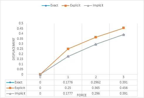
For F (u) =1, u = 0.1776

For F (u) =2, u = 0.2962

For F (u) =3, u = 0.391

Conclusion:

The plot for the results shows that the implicit curve fits well with the exact solution whereas explicit drifts from the exact solution. The Newton Raphson iteration corrects the incremental steps to make it close to the exact one according to the specified tolerance. Also shows that the implicit method has less error when compared to the explicit method, but it is a time-consuming process – explicit method can predict approx. solutions much faster with repeated iterations.

Which is better of the two is entirely depends on the type of the problem and time – accuracy we have.