Week - 2 - Explicit and Implicit Analysis

Introduction:Explicit and Implicit Analysis

Explicit and implicit methods are used in numerical analysis for obtaining numerical approximations to find solutions of time-dependent ordinary and partial differential equations which require computer simulations of physical processes.Explicit methods estimates the state of a system at a later time(i+1) from the state of the system at the current time(i), whereas implicit methods find a solution by solving an equation involving both the current state(i) of the system and the later one(i+1) by using matrix inversion method.For all nonlinear and dynamic analyses, incremental loads are needed. Commonly, ‘implicit’ and ‘explicit’ methods are used to solve these problems.In static analysis, there is no effect of mass (inertia) or of damping (Ku=F). In dynamic analysis, nodal forces associated with mass/inertia and damping are included(Md2U+Cdu+Ku=f). Dynamic analysis can be done through the explicit solver or the implicit solver.In nonlinear implicit analysis, solution of each step requires solution iterations to establish equilibrium within a certain tolerance say (1e-2). In explicit analysis, no iteration is required as the nodal accelerations are solved directly.Implicit and Explicit analysis dissociate in the approach to time incrementation. In Implicit analysis, each time increment has to converge, but you can set quite long time increments. Conversely, explicit analysis doesn’t have to converge each increment, but time increments must be super small for the accuracy of solution.In this work a non linear force equation is used to find for the displacement force relationship by using both explicit and implicit analysis.

When to use Explicit Analysis

Explicit methods should be used when the strain rates/velocity is equal to 10 units/second or more. These events can be illustrated by some examples such as an automotive crash, ballistic explosion, drop and so on. Besides the variation of stress with strain in these cases, also the the strain rate needs to be considered.There is no convergence criteria to check or iteration. The solver focus the calculation of local finite element variables.Solver calculates all of the local finite element variables for given incrementation, and move to the next one.

• Pros: Each increment is calculated extremely fast.
• Cons: The time step has to be super small. Otherwise, it’s impossible to pursue this equilibrium.

When to use Implicit Analysis

Implicit methods should be used when the boundary conditions affect the structure slowly, and the effects of strain rates are small. Once the increment of stress as a function of strain can be established, geometry can be analyzed using implicit methods.The global equilibrium in the model is achieved in each time increment. This means at each increment convergence should be achieved.After global equilibrium is converged, solver calculates all the local finite element variables (stresses, strain, etc.) for each increment.

• Pros: Since global equilibrium is verified at each time increment, those increments can be large.
• Cons: Each time increment is computed slowly, and iterations are needed to get to the global equilibrium.

In order to prove which approach is correct the equation F(u)=u3+9u2+4u is used and solved for internal force and displacement by both approaches Explicit and implicit

`F(u)=u^3+9u^2+4u` Equation of force

`k = 3u^2+18u+4` stiffness

Force displacement relation is given by

`triangleF=k.triangleu` which is similar to the spring equation F=ku where k is the stiffness of the spring `

Explicit Method

To start the problem initial condition for this problem is taken as uo=0. Force displacement relationship is used to find change in the displacement

Step 1

`u0=0`

k(u0)=4

from the stiffness relation

`triangleu=trianglef / k` `triangleu=0.25`

u1=u0+`triangleu`=0.25

f(u0)=1.578 internal force

R=f-F=0.578 residue

for the remaining time step Matlab code is used to solve the equation

% Explicit method
uexp=0
Fexp=1
for j=1:n
  kexp=(3*(uexp^2))+(18*uexp)+4  
   deluexp=delf/kexp
     uexp=uexp+deluexp
    fexp=(uexp^3)+(9*(uexp^2))+(4*uexp)
    Rexp=fexp-Fexp
uexplicit(j)=uexp
fexplicit(j)=fexp
Rexplicit(j)=Rexp
Fexplicit(j)=Fexp
dellexplicit(j)=deluexp
Fexp=Fexp+1
end

Step i	`triangleFi`	`triangleui`	ui	Fext	Finternal	Residue
1	1	0.25	0.25	1	1.5781	0.5781
2	1	0.1151	0.3651	2	2.7088	0.7088
3	1	0.0911	0.4563	3	3.7935	0.7935

From the value of residue, it can be confirmed that in the explicit method force equilibrium is not attained at each step

Implicit Analysis

In implicit analysis, Newton Rapson method is used for each time step to minimize the residue

the initial part of the problem will be similar to the explicit analyisis

Step 1

tolerance=1e-3

`u0=0`

k(u0)=4

from the stiffness relation

`triangleu=trianglef / k` `triangleu=0.25`

u1=u0+`triangleu`=0.25

f(u0)=1.578 internal force

R=f-F=0.578> tolerance residue

Newton Rapson method is used

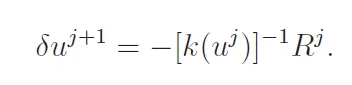
The above equation is obtained by resolving the Taylor series

`deltau=-0.1151*0.578`=-0.0665

`u=u+deltau`=0.1835

f(u)=1.0429

R=0.0429>tolerance

Newton rapson method is used

= -0.0665-(8.6875^-1)*0.0429=-0.0715

u=0.25-0.0715=0.1785

f(u)=1.0066

r=1-1.0066=0.0066>1e-3

rewton rapson method is used

Matlab code is used to solve remaining problem

% Implicit analysis
u=0
delf=1
n=3
tol=1e-3
F=delf
tauu=0
% Implicit analysis
for i=1:n
k=(3*(u^2))+(18*u)+4
delu=delf/k
u=u+delu
f=(u^3)+(9*(u^2))+(4*u)
R=f-F
u0=u
while (abs(R)>=tol)
k=(3*(u0^2))+(18*u0)+4
tauu=tauu-(inv(k)*(R))
u=u0+tauu
f=(u^3)+(9*(u^2))+(4*u)
R=f-F
end
tauux(i)=tauu
uimplicit(i)=u
fimplicit(i)=f
Rimplicit(i)=R
F=F+1
end

Step i	`triangleFi`	`triangleui`	ui	Fext	Finternal	Residue( 1.0e-3)
1	1	0.25	0.1776	1	1.0002	0.1682
2	1	0.1151	0.2961	2	1.9999	-0.1249
3	1	0.0911	0.3910	3	2.9999	-0.1164

The value of residue is closer to zero hence the force equilibrium conditions are maintained

Results :

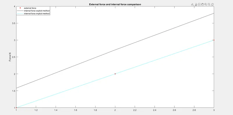
From the graph, it can be inferred that external forces and internal forces using the implicit method coincide with each other whereas in the explicit method there is a gap between external forces and internal forces and this represents the residue.

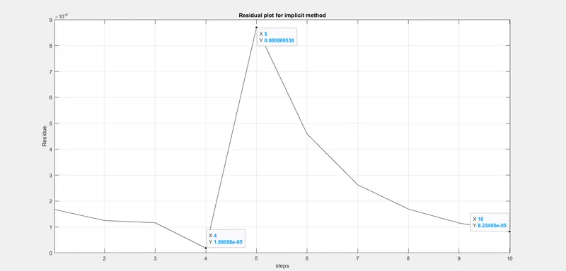
From the graph, it can be inferred that the residue(R=internal force-external force) first gradually decreases with an increase in steps and increases sharply to the step of 5 R=0.000869538 and gradually decreases to 8.234e-5 at the step=10

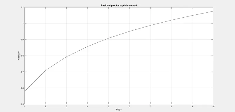
from this graph it can be inferred that the residue increases with the steps in 4th order curve( obtained from curve fitting MATLAB) and reaches the max of 1.07513 at step=10

Conclusion:

Both implicit and explicit methods can be used to solve nonlinear equations. when accuracy is used for comparison implicit method stands first. in the case of time consumption explicit method is preferred over the implicit method.