Week 2 Bevel Gear Challenge
Week 2 Challenge: Bevel Gear Challenge
Course: Introduction to Structural Analysis using ANSYS Workbench
Submitted by: Amanpreet Singh Whan
Supervisor: Vineet G
March 01, 2022
List of Figures
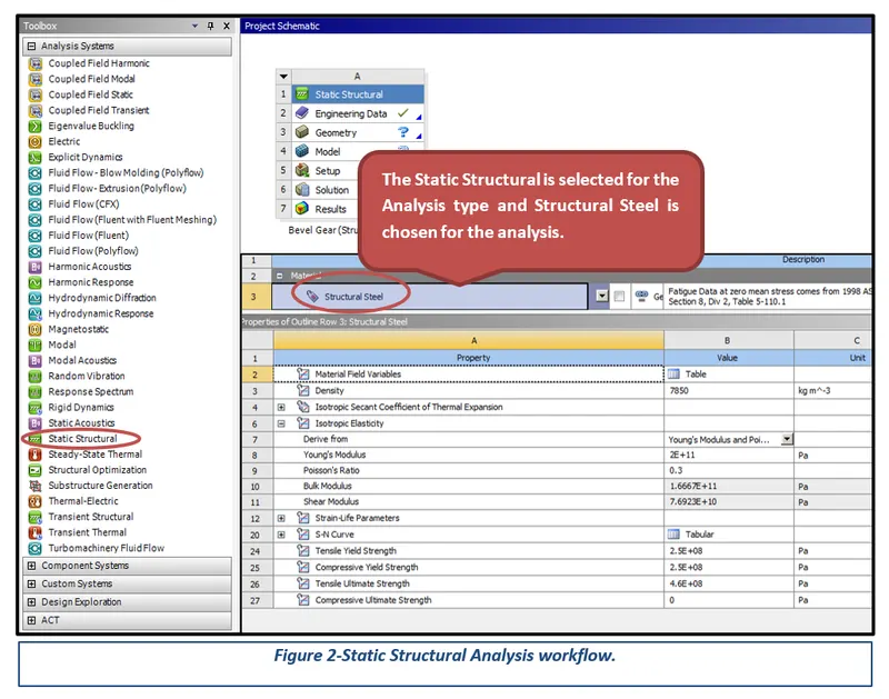
Figure 2-Static Structural Analysis workflow.
Figure 3-Imported given Bevel Gear CAD Model.
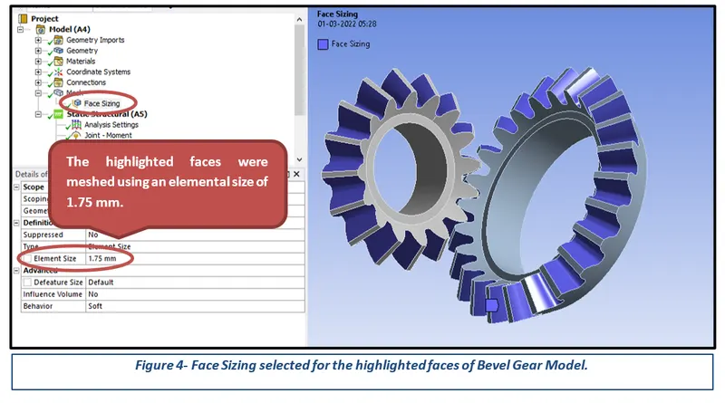
Figure 4- Face Sizing selected for the highlighted faces of the Bevel Gear Model.
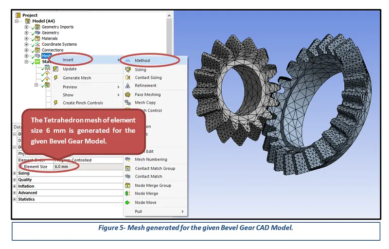
Figure 5- Mesh generated for the given Bevel Gear CAD Model.
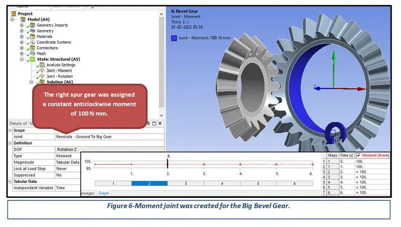
Figure 6-Moment joint was created for the Big Bevel Gear.
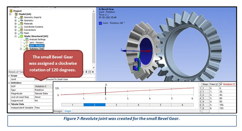
Figure 7-Revolute joint was created for the small Bevel Gear.
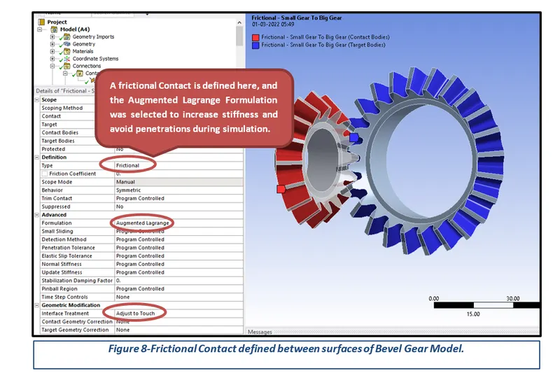
Figure 8-Frictional Contact defined between surfaces of Bevel Gear Model.
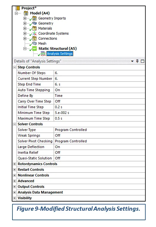
Figure 9-Modified Structural Analysis Settings.
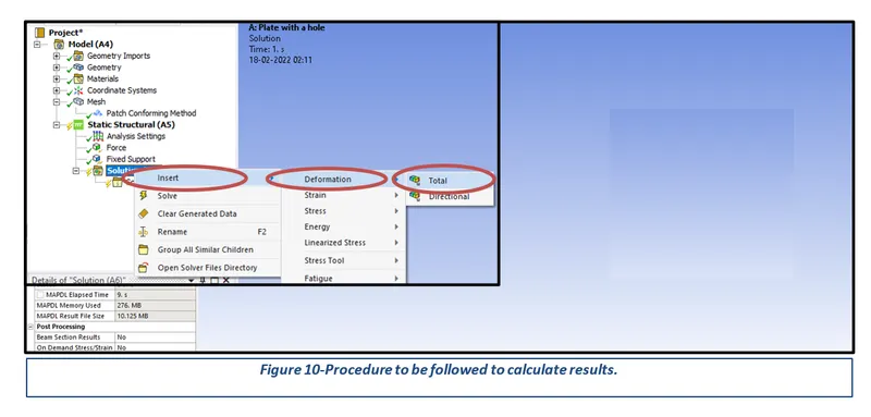
Figure 10-Procedure to be followed to calculate results.
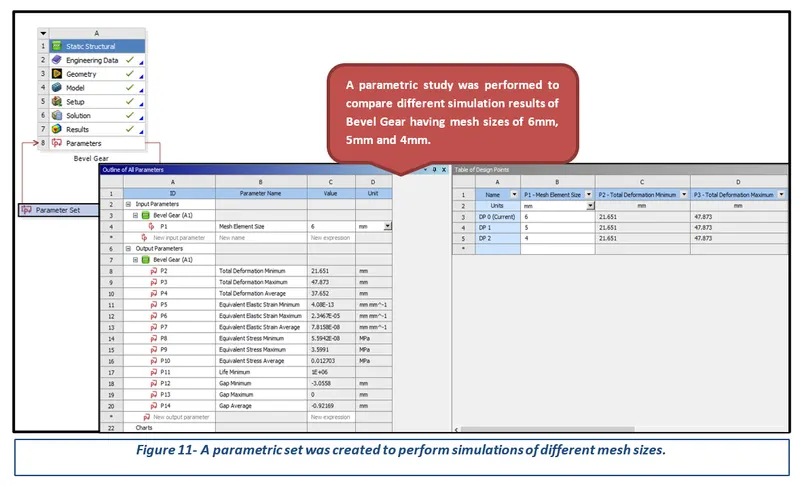
Figure 11- A parametric set was created to perform simulations of different mesh sizes.
Table of Contents
3.1 Importing and Meshing of CAD Model
1 Introduction
ANSYS is a general-purpose, finite-element modeling package for numerically solving a wide variety of mechanical problems. These problems include static/dynamic, structural analysis, heat transfer, and fluid problems, as well as acoustic and electromagnetic problems. There are two methods to use ANSYS. One method is to use the graphical user interface (GUI). This method follows the conventions of popular Windows and X-Windows-based programs. Another method is to use command files. The command-file approach has a steeper learning curve for many, but it has the advantage that the entire analysis can be described in a small text file, typically in less than 50 lines of commands. This approach enables easy model modifications and minimal file-space requirements. The ANSYS environment contains two windows: the main window and an output window. A large number of files are created when ANSYS simulation is run.
Theory
Grid Dependence Test:
The grid dependency test is to investigate how the solution depends on the grid size by running the simulation with refined mesh that is finer the mesh, higher is the accuracy of the result but with additional cost on computation time and computational power. Since solutions are interpolated at the nodes to get an approximate result, the higher the number of nodes and elements is the computational time and power required to complete the simulation.
So, the grid dependency test helps in determining optimal mesh size where the accurate result could be obtained keeping in the mind the cost of time and power. Since the result obtained are approximate. Refining mesh further would result in negligible percent change is the result but only increase the computational cost.
Bevel Gear:
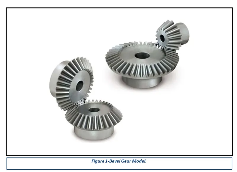
A bevel gear is a toothed rotating machine element used to transfer mechanical energy or shaft power between shafts that are intersecting, either perpendicular or at an angle. This results in a change in the axis of rotation of the shaft power. Aside from this function, bevel gears can also increase or decrease torque while producing the opposite effect on the angular speed. A bevel gear can be imagined as a truncated cone. At its lateral side, teeth are milled which interlock to other gears with its own set of teeth. The gear transmitting the shaft power is called the driver gear, while the gear where power is being transmitted is called the driven gear. The number of teeth of the driver and driven gear is usually different to produce a mechanical advantage. The ratio between the number of teeth of the driven to the driver gear is known as the gear ratio, while the mechanical advantage is the ratio of the output torque to the input torque.
There are different types of bevel gears according to their tooth profile and orientation. The more complicated types such as the spiral and hypoid bevel gears resulted from further development of manufacturing processes such as CNC machining.
Straight Bevel Gear: This is the simplest form of bevel gear. The teeth are in a straight line that intersects at the axis of the gear when extended. The teeth are tapered in thickness making the outer or heel part of the tooth larger than the inner part or toe. Straight bevel gears have instantaneous lines of contact, permitting more tolerance in mounting. A downside to using this type is the vibration and noise. This limits straight bevel gears to low-speed and static loading applications. A common application of straight bevel gears is differential systems in automotive vehicles.
Spiral Bevel Gears: This is the most complex form of bevel gear. The teeth of spiral gears are curved and oblique, in contrast to the teeth orientation of straight bevel gears. This results in more overlap between teeth which promotes gradual engagement and disengagement upon tooth contact. This improved smoothness results in minimal vibration and noise produced during operation. Also, because of higher load sharing from more teeth in contact, spiral bevel gears have better load capacities. This allows them to be smaller in size compared to straight bevel gears with the same capacity.
Zerol Bevel Gears: This type is a modification of a straight bevel gear trademarked by Gleason Works. Zerol bevel gears have teeth curved in the lengthwise direction. These gears are also somewhat similar to spiral bevel gears in terms of their profile. Their difference is the spiral angle; Zerol types have 0° spiral angles while spiral types have 35°.
Hypoid Bevel Gears: This is a special type of bevel gear where the axes of the shafts are not intersecting or parallel. The distance between the two gear axes is called the offset. The teeth of hypoid bevel gears are helical, similar to spiral bevel gears. A hypoid bevel gear designed with no offset is simply a spiral bevel gear. The manufacture and shaping of hypoid types are similar to spiral bevel gears.
2 Aims
- Run rotational simulations for the given Bevel Gear CAD model.
- Apply appropriate Boundary Conditions and simulate for three different mesh sizes of 6mm, 5mm, and 4mm respectively.
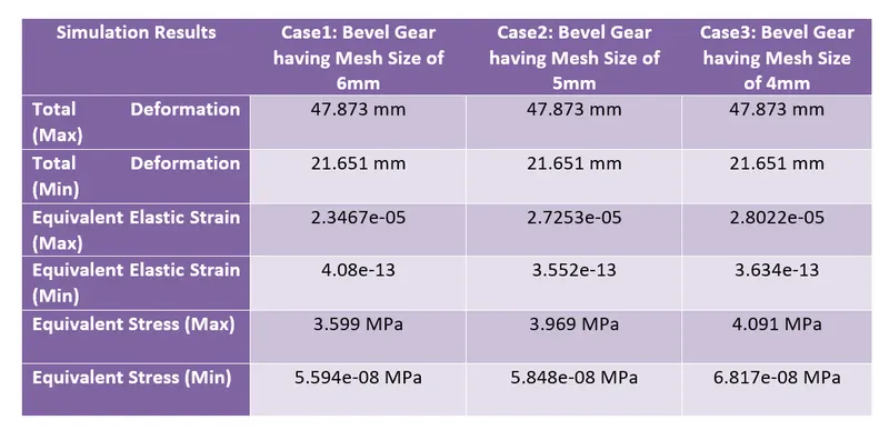
- Determine Total Deformation and Maximum Stress results for the performed simulations and compare the results for the same.
3 Methodology and Results
The section describes the different stages that were performed using an engineering tool Ansys Workbench 2022 for the completion of the Week 2 Challenge. These stages can be further broadly sub-categorized into three key steps, importing the CAD model to apply the boundary conditions and finally performing the simulation to obtain the desired results.
3.1 Importing and Meshing of CAD Model
After opening the Ansys Workbench, the first step is to select the Analysis type and then define appropriate material from the Engineering Data options for the given CAD model. Considering the challenge requirements, Static Structural was selected for the System Analysis type. In addition, three different material cards were created to perform the simulations for the given Bevel Gear CAD Model and are presented in the following figures.
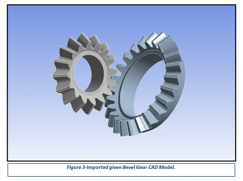
After updating the CAD model in the Ansys Workbench, the next step is to generate a good quality mesh. Meshing is a phase where the CAD geometry is discretized to represent the computational domain in which the solver will discover a solution. A refined mesh helps to achieve better results. The mesh was generated in two steps: a face sizing method with an element size of 1.75 mm was used to refine the faces in contact; for other areas, the mesh was generated using an element size of 6mm.
3.2 Joints
A joint is a type of connection or junction at which usually two bodies are joined together in a way that restricts some degrees of freedom (DOFS) while leaving others free. For a joint, one reference is considered the stationary reference, while the other is considered the mobile or moving reference. The mobile and stationary references of the joint must be on two different bodies. Joints can also be defined as “grounded”. In this case, the joint connects the mobile reference to a fixed location in space. The stationary references are fixed in space, that is they have all DOFs fixed. Properties of a joint are defined as a joint behavior and can be applied to more than one joint. Joint behavior is characterized by the rotational and translational degrees of freedom of the mobile reference of the joint, as fixed or free with reference to the stationary one.
The following figures represent the two revolute joints created; one was given a clockwise rotational motion while the other was provided an anticlockwise moment as per the challenge requirements.
3.3 Contact
In structural analysis software, the contact is generated by pair. Three different contact behaviors are available. They are named node to node (point to point), node to the surface (point to the surface), and surface to surface. As default in Ansys software, point to surface and surface to surface contact types are used. For the point to surface contact, the “point” is contact, and the “surface” is the target. Several contact types are used. These names might be called with different names according to software. In Ansys software, contact names are titled frictional, frictionless, rough, bonded, and have no separation. The Frictional Contact was defined for the challenge purposes and is represented in the following figure.
3.4 Analysis Settings
The given spur gear model was assumed to be simulated for a rotation of 120 degrees to determine appropriate total deformation and other stress-strain results. Therefore, the problem was divided into 6 steps and the Large Deflection option was turned on to prevent Penetration and Intersection errors. The following figure represents the modifications performed in the analysis settings.
Simulation Results
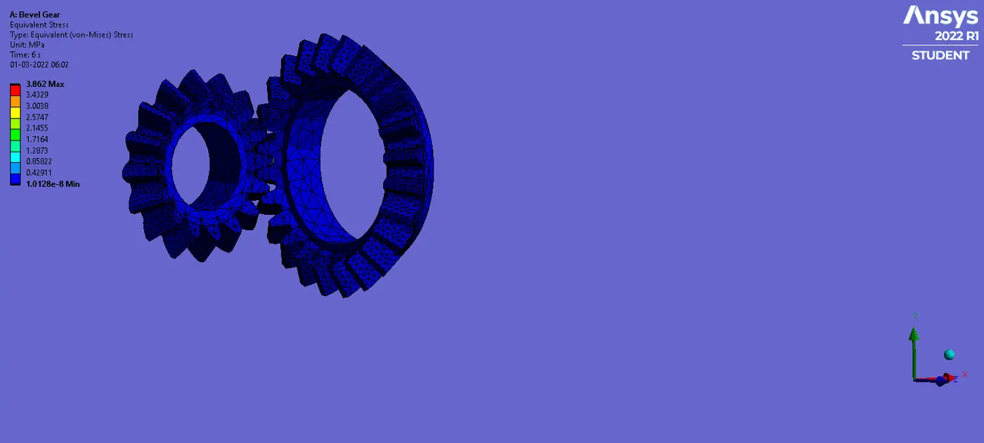
To visualize the simulation or results, the desired output cards have to be created. Total Deformation, Equivalent Elastic Strain, and Equivalent Stress (Von Mises Stress) cards were created using the procedure illustrated in the following picture. It must be noted that the results have to be generated by running the solve command.
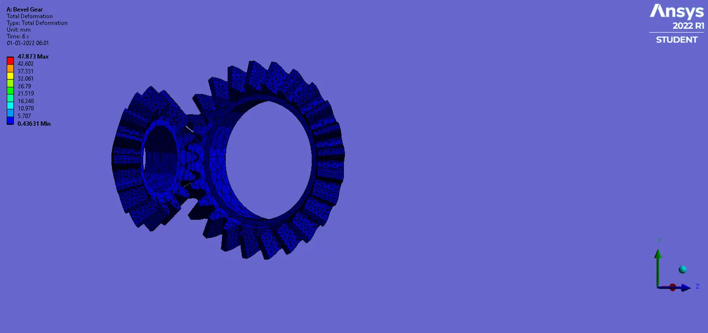
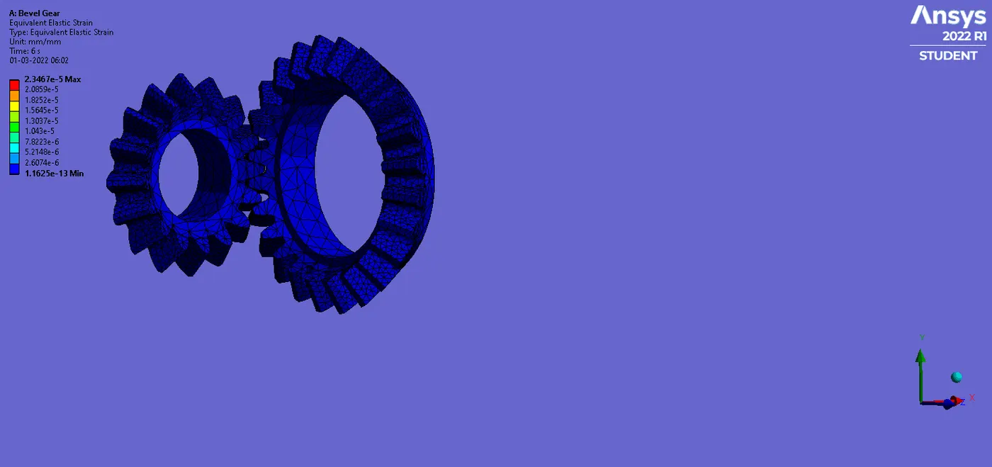
A parametric study was created to find and compare the simulation results of Bevel Gear with different mesh sizes of 6mm, 5 mm and 4 mm. The created parametric set is highlighted in the following figure.
4 Conclusion
In conclusion, the main aim of the Week 2 challenge was to generate a mesh of three different sizes, apply Boundary Constraints and run the simulation and compare the obtained results for the same. It was found that the total deformation in all cases is identical. However, the stresses and strains generated in case 1 and case 2 are smaller in comparison to case 3. Considering the above aspects, it would be not wrong to say that the refinement of the Bevel Gear mesh model yields better stress-strain and more realistic results.