Week 2 Air standard Cycle

• The working fluid is air
• Air behaves as an ideal gas
• Combustion processes are replaced by well-defined heat addition processes
• The exhaust process is replaced by a heat rejection process
• In an air standard cycle, a specific mass of air goes through a complete thermodynamic cycle.

Otto cycle:

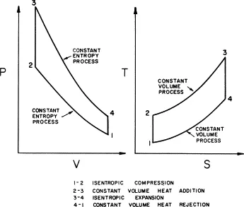
The Otto cycle is a thermodynamic process that describes the changes that occur to a gas in a typical internal combustion engine. The cycle involves a series of changes in pressure, temperature, volume, and heat exchange, ultimately converting fuel into motion.

Solution:

Python code:

import math
import matplotlib.pyplot as plt

def engine_kinematics(bore, stroke, con_rod, cr, start_crank, end_crank):
    """
    Engine kinematics
    """
    # Geometric parameters
    a = stroke / 2
    R = con_rod / a
    # Volume parameters
    V_s = math.pi * (1 / 4) * pow(bore, 2) * stroke
    V_c = V_s / (cr - 1)

    sc = math.radians(start_crank)
    ec = math.radians(end_crank)

    num_values = 50
    dtheta = (ec - sc) / (num_values - 1)
    V = []
    for i in range(num_values):
        theta = sc + i * dtheta
        term1 = 0.5 * (cr - 1)
        term2 = R + 1 - math.cos(theta)
        term3 = pow(R, 2) - pow(math.sin(theta), 2)
        term3 = pow(term3, 0.5)

        V.append((1 + term1 * (term2 - term3)) * V_c)

    return V

# Inputs
p1 = 101325
t1 = 500
gamma = 1.4
t3 = 2300

# Geometric parameters
bore = 0.1
stroke = 0.1
con_rod = 0.15
cr = 12

# Volume computation
v_s = (math.pi / 4) * pow(bore, 2) * stroke
v_c = v_s / (cr - 1)
v1 = v_c + v_s

# State point 2
v2 = v1 / cr
p2 = p1 * pow(v1, gamma) / pow(v2, gamma)

rhs = p1 * v1 / t1
t2 = p2 * v2 / rhs

V_compression = engine_kinematics(bore, stroke, con_rod, cr, 180, 0)
constant = p1 * pow(v1, gamma)
P_compression = [constant / pow(v, gamma) for v in V_compression]

# State point 3
v3 = v2
rhs = p2 * v2 / t2
p3 = rhs * t3 / v3

V_expansion = engine_kinematics(bore, stroke, con_rod, cr, 0, 180)
constant = p3 * pow(v3, gamma)
P_expansion = [constant / pow(v, gamma) for v in V_expansion]

# State point 4
v4 = v1
p4 = p3 * pow(v3, gamma) / pow(v4, gamma)
p4v4_over_t4 = rhs
t4 = p4 * v4 / p4v4_over_t4

# Calculate thermal efficiency
efficiency = [(p * v - p1 * v1) / (t3 - t2) for p, v in zip(P_expansion, V_expansion)]

# Plot PV diagram for Otto cycle
plt.figure(1)
plt.plot([v2, v3], [p2, p3], label='Expansion')
plt.plot(V_compression, P_compression, label='Compression')
plt.plot(V_expansion, P_expansion, label='Expansion')
plt.plot([v4, v1], [p4, p1], label='Compression')
plt.title('Otto Cycle PV Diagram')
plt.xlabel('Volume (m^3)')
plt.ylabel('Pressure (Pa)')
plt.legend()

# Plot thermal efficiency
plt.figure(2)
plt.plot(V_expansion, efficiency)
plt.title('Thermal Efficiency')
plt.xlabel('Volume (m^3)')
plt.ylabel('Efficiency')
plt.show()

Code Explanation:

Import Libraries:

import math import matplotlib.pyplot as plt

• The math module is imported to access mathematical functions like pow, pi, cos, sin, etc.
• matplotlib.pyplot is imported as plt for plotting graphs.

Define function:

def engine_kinematics(bore, stroke, con_rod, cr, start_crank, end_crank): """ Engine kinematics """

• Defines a function named engine_kinematics which calculates the volume variation during the engine cycle based on the geometric parameters and crank angles provided as input.

Calculate Geometric Parameters and Volume:

a = stroke / 2 R = con_rod / a V_s = math.pi * (1 / 4) * pow(bore, 2) * stroke V_c = V_s / (cr - 1)

• Calculates the geometric parameters a and R based on the piston stroke and connecting rod length.
• Computes the stroke volume V_s and clearance volume V_c using the cylinder bore diameter, stroke length, and compression ratio.

Convert Crank Angles to Radians:

sc = math.radians(start_crank) ec = math.radians(end_crank)

• Converts the start and end crank angles from degrees to radians using the radians function from the math module.

Iteratively Calculate Cylinder Volume:

num_values = 50 dtheta = (ec - sc) / (num_values - 1) V = [] for i in range(num_values): theta = sc + i * dtheta term1 = 0.5 * (cr - 1) term2 = R + 1 - math.cos(theta) term3 = pow(R, 2) - pow(math.sin(theta), 2) term3 = pow(term3, 0.5) V.append((1 + term1 * (term2 - term3)) * V_c)

• Determines the number of data points (num_values) and calculates the angle increment (dtheta).
• Loops through the crank angles to compute the cylinder volume at each angle using kinematic equations.
• Appends the calculated volumes to a list V.

Return Cylinder Volumes:

return V

• Returns the list of calculated cylinder volumes.

Define Inputs and Geometric Parameters:

p1 = 101325 t1 = 500 gamma = 1.4 t3 = 2300 bore = 0.1 stroke = 0.1 con_rod = 0.15 cr = 12

• Specifies the initial pressure (p1), initial temperature (t1), adiabatic index (gamma), and temperature at state point 3 (t3).
• Defines the geometric parameters: cylinder bore diameter, piston stroke length, connecting rod length, and compression ratio.

Calculate Total Initial Volume:

v_s = (math.pi / 4) * pow(bore, 2) * stroke v_c = v_s / (cr - 1) v1 = v_c + v_s

• Computes the stroke volume v_s, clearance volume v_c, and total initial volume v1.

State Point 2: Compression Stroke:

v2 = v1 / cr p2 = p1 * pow(v1, gamma) / pow(v2, gamma) rhs = p1 * v1 / t1 t2 = p2 * v2 / rhs

• Calculates the volume (v2) and pressure (p2) at state point 2 based on the compression ratio.
• Computes the temperature (t2) at state point 2 using the energy balance equation.

Compression Stroke Volume and Pressure:

V_compression = engine_kinematics(bore, stroke, con_rod, cr, 180, 0) constant = p1 * pow(v1, gamma) P_compression = [constant / pow(v, gamma) for v in V_compression]

• Calls the engine_kinematics function to simulate the compression stroke and compute the cylinder volumes during compression.
• Computes the pressure at each volume point during compression.

State Point 3: Expansion Stroke:

v3 = v2 rhs = p2 * v2 / t2 p3 = rhs * t3 / v3 V_expansion = engine_kinematics(bore, stroke, con_rod, cr, 0, 180) constant = p3 * pow(v3, gamma) P_expansion = [constant / pow(v, gamma) for v in V_expansion]

• Determines the volume (v3) and pressure (p3) at state point 3.
• Calls the engine_kinematics function to simulate the expansion stroke and compute the cylinder volumes during expansion.
• Computes the pressure at each volume point during expansion.

State Point 4: End of Expansion Stroke:

v4 = v1 p4 = p3 * pow(v3, gamma) / pow(v4, gamma) p4v4_over_t4 = rhs t4 = p4 * v4 / p4v4_over_t4

• Determines the volume (v4) and pressure (p4) at state point 4.
• Computes the temperature (t4) at state point 4 using the energy balance equation.

Calculate Thermal Efficiency:

efficiency = [(p * v - p1 * v1) / (t3 - t2) for p, v in zip(P_expansion, V_expansion)]

• Computes the thermal efficiency of the engine at each stage of the expansion stroke.

Plot PV Diagram for Otto Cycle:

• Creates a new figure (Figure 1) for plotting the PV diagram of the Otto cycle.
• Plots the compression stroke (state points 1 to 2), expansion stroke (state points 3 to 4), and clearance lines.
• Adds a title and labels to the plot for clarity.

Plot Thermal Efficiency:

# Plot thermal efficiency plt.figure(2) plt.plot(V_expansion, efficiency) plt.title('Thermal Efficiency') plt.xlabel('Volume (m^3)') plt.ylabel('Efficiency')

• Creates a new figure (Figure 2) for plotting the thermal efficiency of the engine.
• Plots the thermal efficiency against the cylinder volume during the expansion stroke.
• Adds a title and labels to the plot for clarity.

Display Plots:

plt.show()

Displays the plotted figures (PV diagram and thermal efficiency plot) on the screen.

Output:

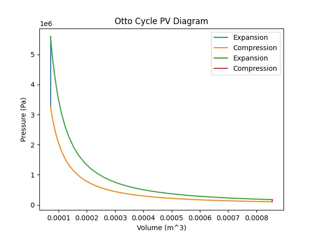
Otto Cycle PV Diagram:

• The plot shows the pressure (Pa) on the y-axis and the volume (m^3) on the x-axis.
• Two main processes are depicted: compression (from state point 1 to 2) and expansion (from state point 3 to 4).
• The compression stroke is represented by the line connecting state points 1 and 2, where the volume decreases and the pressure increases.
• The expansion stroke is represented by the line connecting state points 3 and 4, where the volume increases and the pressure decreases.
• The compression and expansion strokes are shown in different colors for clarity.
• The points where the compression and expansion strokes start and end (state points 1, 2, 3, and 4) are marked on the plot.
• The legend indicates which line corresponds to compression and which one corresponds to expansion.

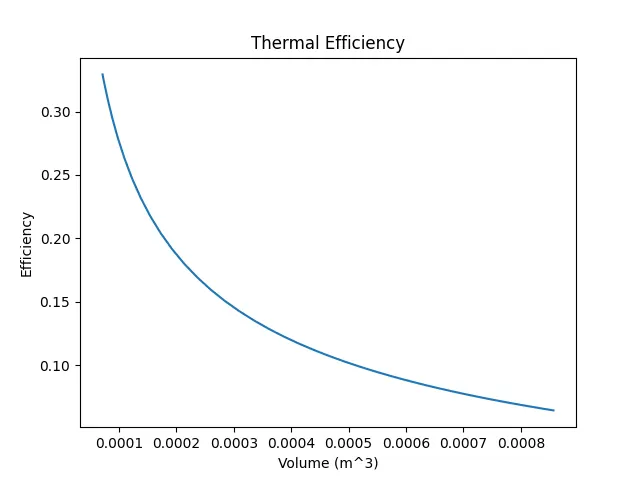
Thermal Efficiency Plot:

• The plot shows the thermal efficiency of the engine against the volume during the expansion stroke.
• The efficiency is calculated based on the difference in work done during expansion and compression strokes and the heat input into the system.
• The x-axis represents the volume (m^3), and the y-axis represents the thermal efficiency.
• The efficiency increases as the volume increases during the expansion stroke, indicating that more work is extracted from the expanding gases.

Conclusion:

• Using python we are created the Otto cycle pv diagram and Thermal efficiency plotted successfully.