Week 2 Air standard Cycle

AIM :-

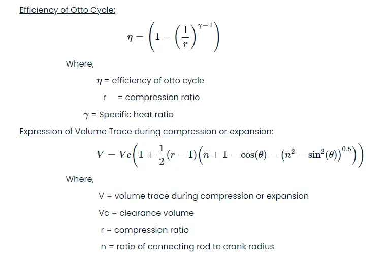
The main aim of this project is to calculate the thermal efficiency of the Otto cycle and create its PV diagram using Python code. Here, while writing the code, it has assumed that the parameters like air inlet pressure and temperature, the maximum temperature at the end of heat addition were already known.

Theory :-

Otto cycle is also called a constant volume cycle where the combustion occurs at constant volume. It has two isentropic processes and two isochoric processes.

                  Where,

                               1 to 2 is isentropic compression

                               2 to 3 is isochoric heat addition

                               3 to 4 is isentropic expansion

                               4 to 1 is isochoric heat rejection

and Vs and Vc are stroke and clearance volumes respectively

PYTHON CODE :-

#Otto cycle simulator

import math
import matplotlib.pyplot as plt

def engine_kinematics(bore,stroke,con_rod,cr,start_crank,end_crank):


		#Geometric parameters
	bore = 0.1    	#Bore dia in mts
	stroke = 0.1  	#Stroke length in mts
	con_rod = 0.15 	#length of connecting rod in mts
	cr = 7        	#Compression ratio
	r = stroke/2    #radius of crank in mts
	n = con_rod/r   #ratio of connecting rod length to crank radius

	#Stroke and Clearence volumes
	vs = (math.pi/4)*pow(bore,2)*stroke  # Stroke Volume
	vc = vs/(cr-1)                       #Clearence volume

	sc = math.radians(start_crank)
	ec = math.radians(end_crank)

	number_values = 50
	dtheta = (ec-sc)/(number_values-1)

	V = []

	for i in range(0,number_values):
		theta = sc + i*dtheta


		#Defining the volume trace equation in parts
		term1 = 0.5*(cr - 1)
		term2 = n + 1 - math.cos(theta)
		term3 = pow(n,2) - pow(math.sin(theta),2)
		term3 = pow(term3, 0.5)

		V.append((1 + term1*(term2 - term3))*vc)

	return V

	#inputs for otto cycle
p1 = 101325 	#Initial pressure in pascals
t1 = 500    	#Initial temperature in kelvin
t3 = 2300       #Temperature after combustion in kelvin
gamma = 1.4     #Specific heat ratio

#Geometric parameter
bore = 0.1    	#Bore dia in mts
stroke = 0.1  	#Stroke length in mts
con_rod = 0.15 	#length of connecting rod in mts
cr = 7      	#Compression ratio

#Clearance and stroke volumes
vs = (math.pi/4)*pow(bore,2)*stroke  # Stroke Volume
vc = vs/(cr-1)  #Clearence volume
v1 = vs + vc    #Volume at state point 1

#State point 2
v2 = vc
p2 = p1*pow(v1,gamma)/pow(v2,gamma)  #p2v2^gamma = p1v1^gamma
c  = p1*v1/t1
t2 = p2*v2/c   #p2v2/t2 = p1v1/t1 = c
V_compression = engine_kinematics(bore,stroke,con_rod,cr,180,0)
constant = p1*pow(v1,gamma)

P_compression = []

for i in V_compression:
	P_compression.append(constant/pow(i,gamma))


#State point 3
v3 = v2
c1 = p2*v2/t2   #p2v2/t2 = p3v3/t3 = c1
p3 = c1*t3/v3
V_expansion = engine_kinematics(bore,stroke,con_rod,cr,0,180)
constant = p3*pow(v3,gamma)

P_expansion = []

for j in V_expansion:
	P_expansion.append(constant/pow(j,gamma))

# State point # 4
v4 = v1
p4 = p3*pow(v3,gamma)/pow(v4,gamma)
t4 = p4*v4/c1

#Calculation of Otto Cycle efficiency
eff = (1-pow(1/cr,gamma-1))*100
print('Efficiency of Given Otto Cycle is',eff)

#Plotting of state points
plt.plot([v2,v3],[p2,p3])
plt.plot(V_compression,P_compression)
plt.plot(V_expansion,P_expansion)
plt.plot([v4,v1],[p4,p1])
plt.show()

Results & Plots :-

a) PV plot for the given otto cycle is :-

b) Efficiency of the given otto cycle is 54.08% for the given compression ratio and specific heat ratio.