Week 2 Air standard Cycle

Otto cycle simulator using Python programming

Otto cycle is a power cycle with constant volume heat addition and constant volume heat rejection. Various processes in it are shown in the below-given figure

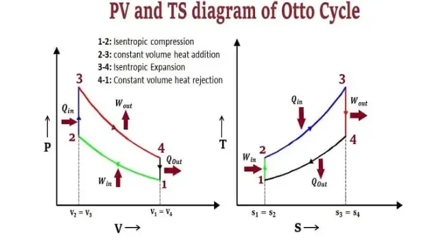
Fig: PV and TS diagram of an Otto cycle

The code to simulate the Otto cycle is written using bore, stroke, compression ratio, connecting rod length, ambient pressure, and temperature as inputs. Further, a function with these variables was created to get an array of volumes and pressures corresponding to various crank angle values.

code

#otto cycle simulator 
#written by Abhishek Kumar

import math
import matplotlib.pyplot as plt
# part 1 defining a function to caluclate volume based on crank angle
#define engine variables

bore= 0.1
stroke=0.1
con_rod= 0.15
#compression ratio 
cr= 12
#crank angles
gamma= 1.4
#swept volume
vs= math.pi*(1/4)* pow(bore,2)* stroke
# clearance volume 
vc= vs/(cr-1)


def engine_kinematics(bore, stroke, con_rod, cr,start_crank, end_crank):
	a= stroke/2
	# parameter R used in the formula v/vc= 1+1/2*(cr-1)*[R+1-cos(theta)-(R^2-sin^2(theta))^1/2]
	R= con_rod/a 
	#defining start and end crank angles
	sc= math.radians(start_crank)
	ec= math.radians(end_crank)
	num_values=50
	dtheta= (ec-sc)/(num_values-1)
	v=[]
	for i in range(0,num_values):
		theta= sc+i*dtheta
	
		# next, using the formula by breaking it into several terms v/vc= 1+1/2*(cr-1)*[R+1-cos(theta)-(R^2-sin^2(theta))^1/2]
		term1= 0.5*(cr-1)
		term2= R+1-math.cos(theta)
		term3= pow(pow(R,2)-pow(math.sin(theta),2),0.5)
		#Assembling all the terms
		volume= vc*(1+term1*(term2-term3))
		v.append(volume)
		
	return v

#this function will be used to calculate array of volume and pressure during compression and expansion processes

# now we have the values of volumes as an array for start and end crank angles
#next, we need to calculate pressure for all the states

# for state point1 we assume atmospheric pressure and abbient temp in kelvin

p1= 101325
t1=500

v1= vc+vs 
#state2

v2= vc

p2= p1* pow(v1,gamma)/pow(v2,gamma)

# finding temperature | p2v2/t2= p1v1/t1 | 

t2= p2*v2*t1/(p1*v1)

v_compression= engine_kinematics(bore, stroke, con_rod, cr, 180, 0)
p_compression=[]
for v in v_compression:
	#using p1v1^gamma=p2v2^gamma
	p_compression.append(p1* pow(v1,gamma)/pow(v,gamma))
	

#state3
#state variables at point 3 | v3= v2 as constant volume heat addition | p3*v3/t3= p2*v2/t2 | assuming t3 = 2300 K
t3= 2300
v3= v2

p3 = (p2*v2*t3)/(v3*t2)
# print(p3>p2)

# computing point 4

v4=v1

# for process 3 to 4 ; p4v4^gamma= p3v3^gamma

p4= p3*pow(v3,gamma)/ pow(v4,gamma)

t4 = (p4*v4*t3)/(p3*v3)

#getting array for the expansion process
v_expansion= engine_kinematics(bore, stroke, con_rod, cr,0, 180)

p_expansion=[]

for v in v_expansion:
	p_expansion.append(p3*pow(v3,gamma)/ pow(v,gamma))

#All the state variables have been calculated| plot the graph now

#calculating efficiency of the otto cycle
# efficiency= 1-(v2/v2)^(gamma-1)

efficiency= (1-pow((v2/v1),(gamma-1)))*100
print('otto cycle efficiency:')
print(efficiency, '%')

plt.plot([v2,v3], [p2,p3]) 
plt.plot(v_compression, p_compression)
plt.plot(v_expansion, p_expansion)
plt.plot([v4,v1], [p4,p1]) 
plt.xlabel('volume (M^3)')
plt.ylabel('pressure(MPA)')
plt.show()
"""
output: 
otto cycle efficiency:
62.98928275128466 %
"""

Plot Generated as output:

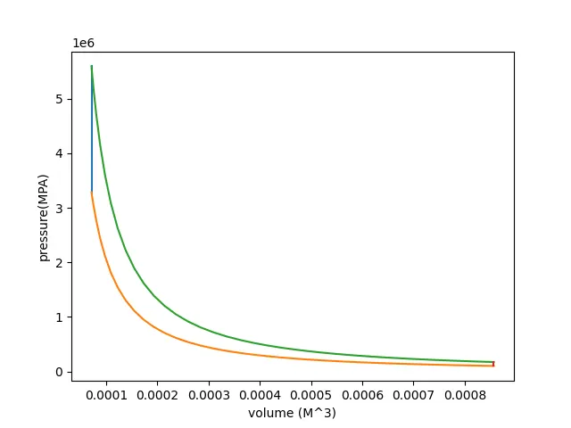
Fig: The P-V diagram of otto cycle

The efficiency of the Otto cycle was calculated using the formula: `eta= 1-((v2)/(v1))^(gamma-1`

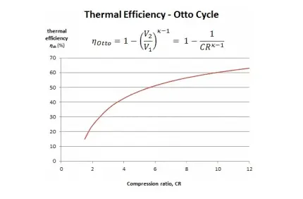
Fig: plot for thermal efficiency of Otto cycle with respect to compression ratio

Since the compression ratio in this project was 12, the efficiency of 62% is in agreement of the general trend