Week 2 Air standard Cycle

AIR STANDARD CYCLE:

Aim:

to write a code to solve the otto cycle and to plot the graph.

Introduction:

An Otto cycle is an idealized thermodynamic cycle that describes the functioning of a typical spark ignition piston engine. It is the thermodynamic cycle most commonly found in automobile engines.

The Otto cycle is a description of what happens to a gas as it is subjected to changes of pressure, temperature, volume, addition of heat, and removal of heat. The gas that is subjected to those changes is called the system. The system, in this case, is defined to be the fluid (gas) within the cylinder. By describing the changes that take place within the system, it will also describe in inverse, the system's effect on the environment. In the case of the Otto cycle, the effect will be to produce enough net work from the system so as to propel an automobile and its occupants in the environment.

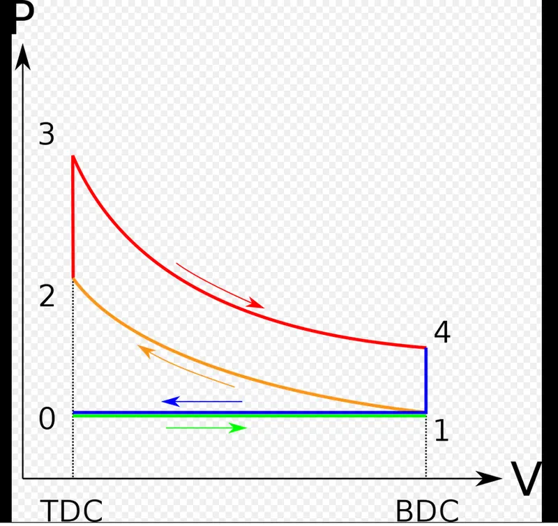
pv diagram.

there are four process taking place in otto cycle

process 1-2 reversible abiabatic compression.

process 2-3 constant volume heat addition.

proces 3-4 reversible abiabatic expansion.

process 4-1 constant volume heat rejection.

formulas used for otto cycle:

for proces 1-2:

reversible adiabatic compression:

adiabatic process

p*v^gamma=constant

p1*v1^gamma=p2*v2^gamma

for process 2-3:

constant volume heat addition process:

v2=v3;

(p2*v2)/t2=(p3*v3)/t3

p2/p3=t2/t3

for proces 3-4:

reversible adiabatic expansion:

adiabatic process

p*v^gamma=constant

p3*v3^gamma=p4*v4^gamma

for process 4-1:

constant volume heat addition process:

v4=v1;

(p4*v4)/t4=(p1*v1)/t1

p4/p1=t4/t1

by using the above formulas we can calculate the p,v,t of all the points 1,2,3,4.

to get a graph of otto cycle. we need to use kinematic psiton formula to obtain the graph:

v=vc*(1+0.5*(rc-1)[R+1-cos(theta)-(R^2-sin(theta)^0.5])

for writing script:

given data:

p1=101325 pa,t1=500k, t3=2300k, bore=0.1m, sroke=0.1m, con_rod=0.5m, compression ratio=12 and gamma=1.4

python script::

import math as m
import numpy as np
import matplotlib.pyplot as plt

def engine_kinematic(con_rod,stroke,v_c,c_r,sc,ec):
	a=stroke/2
	r=con_rod/a
	v_s=(m.pi/4)*pow(bore,2)*stroke
	v_c=v_s/(c_r-1)

	s_c=m.radians(sc)
	e_c=m.radians(ec)

	theta=np.linspace(s_c,e_c,50)

	v=[]

	for i in range(0,50):
		Theta=theta[i]
		term1=0.5*(c_r-1)
		term2=r+1-(m.cos(Theta))
		term3=pow(r,2)-pow(m.sin(Theta),2)
		term4=pow(term3,0.5)

		v.append(v_c*(1+term1*(term2-term4)))

	return(v)

# given parameter:
p1=101325 #pressure in pascal
t1=500 #temperature in k 
t3=2300  #maximum temperature in k
bore=0.1 #bore diameter(m)
stroke=0.1  #stroke length(m) 
con_rod=0.5 #connecting rod length (m) 
c_r=12  
gamma=1.4


#to calculate swept volume,clearance volume.
v_s=(m.pi/4)*pow(bore,2)*stroke
v_c=v_s/(c_r-1)

#to calculate v1,v2
v1=v_s+v_c 
v2=v_c
v3=v2
v4=v1
c=p1*pow(v1,gamma)

#process 1-2: reversible abiabatic compression:
#p1*v1^gamma=p2*v2^gamma
p2=p1*pow((v1/v2),gamma)
#t1/t2=(v2/v1)^gamma-1
t2=t1*pow((v1/v2),(gamma-1))  #we got p1,v1,t1,p2,v2 and t2

#process 2-3: constant volume heat addition
#p2/t2=p3/t3
p3=(p2*t3)/t2 ##we got p3,v3 and t3

#process 3_4 reversible adiabatic expansion:
#p3*v3^gamma=p4*v4^gamma
p4=p3*pow((v3/v4),gamma)
#t1/t2=(v2/v1)^gamma-1
t4=t3*pow((v3/v4),(gamma-1)) # we got p4,v4, t4
e=p4*pow(v4,gamma)
# for compression:
v_compression=engine_kinematic(con_rod,stroke,v_c,c_r,180,0)

p_compression=[]
for i in range(0,50):
	v=v_compression[i]
	p_compression.append(c/(pow(v,gamma)))

#for expansion:
v_expansion=engine_kinematic(con_rod,stroke,v_c,c_r,0,180)
p_expansion=[]
for i in range(0,50):
	v=v_expansion[i]
	p_expansion.append(e/pow(v,gamma))


#to calcualte the thermal efficiency:
#thermal efficiency= (heat addition-heat rejection)/heat addition

heat_addition=t3-t2
heat_rejection=t4-t1
thermal_efficiency= ((heat_addition-heat_rejection)/heat_addition)*100
print('thermal efficiency of otto cycle is',thermal_efficiency)	

#plotting:
plt.plot(v_compression,p_compression)
plt.plot(v_expansion,p_expansion)
plt.plot([v1,v4],[p1,p4])
plt.plot([v2,v3],[p2,p3])
plt.legend(['Reversible Adiabatic Compression','Constant volume Heat addition','Reversible Adiabatic Expansion','Constant Heat rejection'])
plt.xlabel('volume(m^3)')
plt.ylabel('pressure(pa)')
plt.title('otto cycle for pv diagram')
plt.text(v1,-3*pow(10,4),'1')
plt.text(v2,p2,'2')
plt.text(v3,p3,'3')
plt.text(v1,3.5*pow(10,5),'4')
plt.show()

procedure explanation:

first, we have to define the engine geomentric parameter like bore dia, stroke length, connecting rod length,critical ratio.

then write a code for piston kinematic function.

then calculate the all four state values like p,v and t.

by using the point , plot the pv diagram of otto cycle.

now, run the script to plot the pv diagram.

output:

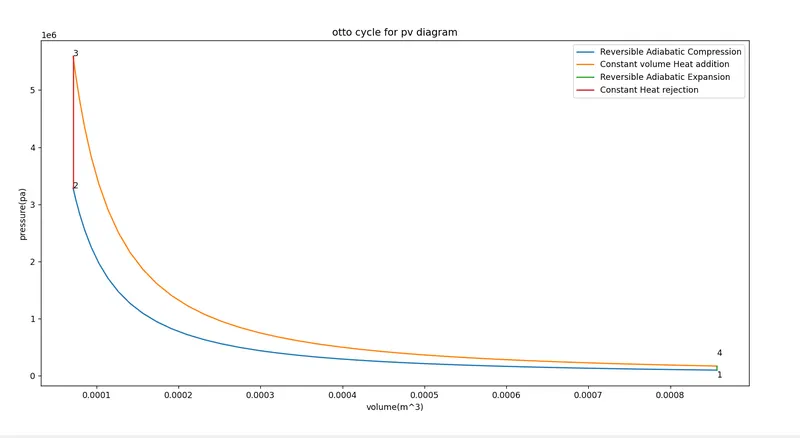
pv diagram of otto cycle.

calculation for thermal efficiency:

thermal efficiency=((heat_addition-heat_rejection)/heat_addition)*100

heat addition =m*cv*dt =m*cv*(t3-t2)

heat rejection =m*cv*dt =m*cv*(t4-t1)

results:

Here are the requirements

1. Your code should create a PV diagram

2. You should output the thermal efficiency of the engine.

the above has been done.

----------------------------------thank you-------------------------------------------