Week 2 Air standard Cycle

Aim:- To create a P-V diagram of otto cy and calculating thermal efficiency of it by using python

Objective:-

• Create a P-V diagram
• Calculating thermal efficiency of the engine

Theory:-

Air Standard Cycle –

The air standard cycle is a thermodynamic power cycle that converts heat energy into mechanical power by considering air as a working fluid with constant specific heats. In this cycle, the air is the only working fluid that goes through changes in its thermodynamic properties to convert heat into mechanical power. There are four types of air standard cycles are Otto cycle, Diesel cycle, Dual cycle and Brayton cycle. In these cycles, we are discussing about Otto cycle.

Assumptions of air standard cycle-

1. Air is taken as gas
2. The compression and expansion process is a adiabatic and reversible
3. The Cycle is considered as a closed system with no air leaving and entering in the system

Otto Cycle –

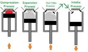
An Otto cycle is an idealized thermodynamic cycle that describes the functioning of a typical spark ignition piston engine. It is the thermodynamic cycle most commonly found in automobile engines. It is based on constant volume heat addition (combustion) and heat rejection processes, and isentropic compression and expansion. This cycle is shown above on P–V diagrams.

The Otto cycle consists of four processes:

Process 1 → 2: Reversible adiabatic compression

Process 2 → 3: Heat addition at constant volume

Process 3 → 4: Reversible adiabatic expansion

Process 4 → 1: Heat rejection at constant volume

Program:-

Engine Geometric parameters:-

Cylinder diameter(bore)- 0.15m

Stroke length- 0.2m

connecting rod length- 0.15

compression ratio- 12

let take,

p1-101325 pa

T1- 500 k

T3- 2000 k

gamma- 1.4

Coding-

import math
import matplotlib.pyplot as plt
import numpy as np

# user defined function
def engine_kinematics (bore,stroke,connecting_rod,c_r,start_crank_angle,end_crank_angle):
	# Engine geometric properties
	a = stroke/2
	R = connecting_rod/a

	# Volume parameters
	v_swept = (math.pi/4)*pow(bore,2)*stroke
	v_clearance = v_swept/(c_r-1)

	# Defining start and end crank angle
	sc = math.radians(start_crank_angle)
	ec = math.radians(end_crank_angle)

	theta =np.linspace(sc,ec,50)
	v = []

	for i in range(0,50):
		Theta = theta[i]
		term_1 = 0.5*(c_r-1)
		term_2 = R+1-math.cos(Theta)
		term_3 = pow((pow(R,2)- pow(math.sin(Theta),2)),0.5)
		v.append((1+term_1*(term_2-term_3))*v_clearance)
	return v


# Input variable
gamma = 1.4 # for air gamma = 1.4
T3 = 2000   # max temp inside engine cylinder

# State variables at inlet to engine
# ambient atmospheric conditions assumed
p1 = 101325
T1 = 500

# Engine geometric parameters
bore = 0.15
stroke = 0.2
connecting_rod = 0.15
c_r = 12

# Calculating swept volume and clearance volume 
v_swept = (math.pi/4)*pow(bore,2)*stroke
v_clearance = v_swept/(c_r-1)
v1=v_swept + v_clearance
v2 = v_clearance

# calculation of p2 and T2
p2 = p1*pow(c_r,gamma)
# (p1*v1)/T1 =(p2*v2)/T2
# T2=p2*v2*T1/(p1*v1)
T2=p2*v2*T1/(p1*v1)

# To find variation of volume during compression stroke as a function of crank angle theta
V_comp = engine_kinematics(bore,stroke,connecting_rod,c_r,180,0)
C_const = p1*pow(v1,gamma)
P_comp = []
print(V_comp)

for v in V_comp:
	P_comp.append(C_const/pow(v,gamma))
print(P_comp)



# Calculation of p3 and v3
# (pv/T=constant)
# for process 2-3 v2 = v3
# (p2/T2)=(p3/T3)
p3 = p2*(T3/T2)
v3 = v2

# To find variation of volume during expansion stroke as a function of crank angle theta
V_exp = engine_kinematics(bore,stroke,connecting_rod,c_r,0,180)
C_const = p3*pow(v3,gamma)
P_exp = []
print(V_exp)

for v in V_exp:
	P_exp.append(C_const/pow(v,gamma))
print(P_exp)


# Calculation of p4,v4 and T4
# p3*v3^gamma = p4*v4^gamma 
v4 = v1
p4 = p3*pow(v3,gamma)/pow(v4,gamma) #Isentropic expansion process

# Plotting
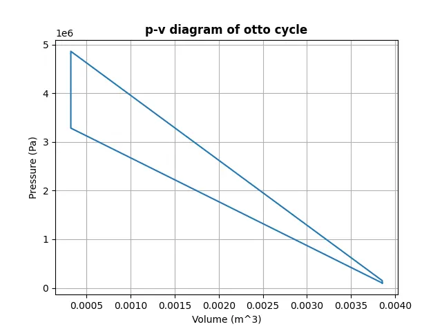
plt.plot([v1,v2,v3,v4,v1],[p1,p2,p3,p4,p1])
plt.xlabel('Volume (m^3)')
plt.ylabel('Pressure (Pa)')
plt.title('p-v diagram of otto cycle', fontweight="bold")
plt.grid()
plt.show()

# Plotting
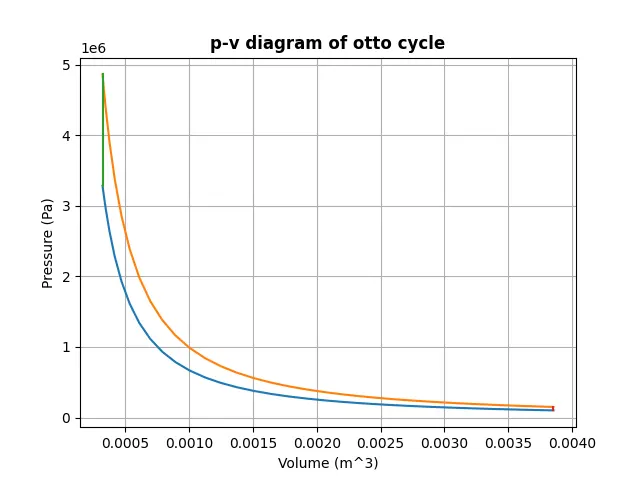
plt.plot(V_comp,P_comp)
plt.plot(V_exp,P_exp)
plt.plot([v2,v3],[p2,p3])
plt.plot([v4,v1],[p4,p1])
plt.xlabel('Volume (m^3)')
plt.ylabel('Pressure (Pa)')
plt.title('p-v diagram of otto cycle', fontweight="bold")
plt.grid()
plt.show()

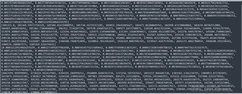
Output- (Compression volume, Compression pressure, Expansion Volume and Expansion pressure)

for Thermal efficiency of otto cycle

# Calculating thermal efficiency of otto cycle

Thermal_efficiency = 1 -(1/pow((c_r),(gamma-1)))
print(Thermal_efficiency)

Output- Thermal efficiency of otto cycle

P-V diagram-

Theoretical diagram-

Actual diagram-

Result:- Otto cycle coding done and PV diagram found satisfactory.