Week 2 Air standard Cycle

Aim:

• To write a code on Otto cycle and calculate its thermodynamic efficiency
• To plot a P-V diagram both actual and theoritical considering engine kinematics formula.

Theory:

Otto cycle is named after Nikolas August Otto. This Otto cycle is also known as constant volume cycle. These cycle generally used in gasoline engines.

Equation Used:

Thermodynamic processes of otto cycle:

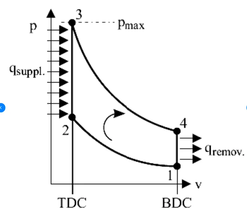
0---1= Suction stroke

1---2= Adiabatic compression

2----3= Contant volume heat addition

3----4= Adiabatic expansion

4----1= Constant volume heat rejection

P,V,T relations used:

1. For P,V------(P2/P1)=(V1/V2)^2
2. For T,V------(T2/T1)=(V1/V2)^(gamma -1)
3. For P,T-------(P2/P1)^(1/gamma)=(T2/T1)^1/(gamma-1)
4. ideal gaas equation = Pv = nRT, where, n= no of moles, R= universal gas constant

The equation of engine kinematics:

Code:

##CODE:
import math
import matplotlib.pyplot as plt
import numpy as np
#defining the Function
def eng_kinematics (bore_dia,stroke_length,connecting_rod_length,r_c,start_crank_angle,end_crank_angle):
    a = stroke_length/2 
    R = connecting_rod_length/a
    v_swept = math.pi*(1/4)*pow(bore_dia,2)*stroke_length
    v_clearence = v_swept/(r_c-1)

    start_crank = math.radians(start_crank_angle)
    end_crank = math.radians(end_crank_angle)
    theta = np.linspace(start_crank,end_crank,50)

    v = []
    num_values = 50
    dtheta = (end_crank - start_crank)/(num_values-1)
    for i in range(0,50):
        theta = start_crank + i*dtheta
        term_1 = 0.5*(r_c-1)
        term_2 = R+1-math.cos(theta)
        term_3 = pow(R,2)-pow(math.sin(theta),2)
        term_3= pow(term_3,0.5)
        v.append((1+term_1*(term_2- term_3))*v_clearence)
    return v


#Defining the input parameters
p1 = 101325
t1 = 500
gamma = 1.4 #adiabatic index for air
#Defining the engine geometric parametrs
bore_dia = 0.8
stroke_length = 0.2
connecting_rod_length = 0.15
r_c = 12 #compression ratio

#calculation of swept volume and clearence volume
v_swept = (math.pi/4)*pow(bore_dia,2)*stroke_length
v_clearence = v_swept/(r_c-1)
v1 = v_swept + v_clearence

#calculation of parameters at point 2
v2 = v_clearence
p2 = p1*pow(v1,gamma)/pow(v2,gamma)
t2 = (p2*v2*t1)/(p1*v1)

#to find the variation during compression stroke, as a function of crank angle  theta,180,0
v_comp = eng_kinematics (bore_dia,stroke_length,connecting_rod_length,r_c,180,0)
c_constant = p1*pow(v1,gamma)
p_comp = []

for v in v_comp:
    p_comp.append(c_constant/pow(v,gamma))


#calculation of parameters at point 3
v3 = v_clearence
t3 = 2300 #temperature during compression
p3 =(p2*v2*t3)/(v3*t2)
#calculation of parameters at point 4
v4 = v1
p4 = p3*pow(v3,gamma)/pow(v4,gamma)
t4 = (p4*v4*t3)/(p3*v3)

#to find the variation during expansion stroke, as a function of crank angle  theta,0,180
v_exp = eng_kinematics(bore_dia,stroke_length,connecting_rod_length,r_c,0,180)
c_constant = p3*pow(v3,gamma)
p_exp = []
for v in v_exp:
    p_exp.append(c_constant/pow(v,gamma))


#calculating the thermal efficiency
Efficiency = 1-(t4-t1)/(t3-t1)
print(Efficiency)

#plotting the p-v digram, without considering engine kinematics equation
plt.plot([v1,v2,v3,v4,v1],[p1,p2,p3,p4,p1],color='g',linewidth='1.5')
plt.xlabel('Voloume in m^3')
plt.ylabel('Pressure in Pa')
plt.title('P-V diagram of Otto Cyle,Theoritical')
plt.legend(["Theoritical"])
plt.grid()
plt.show()
plt.legend(["Theoritical"])
# plotting 
plt.plot(v_comp,p_comp)
plt.plot(v_exp,p_exp)
plt.plot([v2,v3],[p2,p3])
plt.plot([v4,v1],[p4,p1])
plt.xlabel('Voloume in m^3')
plt.ylabel('Pressure in Pa')
plt.title('P-V diagram of Otto Cyle,Actual')
plt.legend(["Isentropic Compression","Isentropic Expansion","Constant Volume Heat Addition","constant Volume Heat Rejection"])
plt.grid()
plt.show()

Code Explaination:

At the begining of this code the required module math, matplotlib and numpy has been called. Initially,the function has been defined name eng_kinematics and the input arguments has also written. The equation of a,R,swept volume,clearence volume derived within the code.After that the start crank angle and end crank angle derived in radians with the help of math module. Then an array for theta has been created with division 50 in command (np.linspace(start_crank,end_crank,50)).Next a for loop has been generated for 50 iterations of crank angle, to calculate the equation of engine kinematics.

After defining function code, all engine parameters has been written, such as bore diameter, stroke lenght, length of the connecting rod,compression ratio. The input parameters such as p1,t1 and t3 has also been written before calling the function. Now to determiine the paramaeters pressure,temperature and volume in each points the P,V,T thermo dynamicc realtion and the ideal gas eqaution has been used at point 2,3,4 respectively. Aftter that to get the curves foe Isentropic or adibatic compression and in expansion the value of each point in those states the funtion has been called(from 2 to 3, and from 3 to 4). neext the thermal efficiency has calculated. Then to get the Theoritical pv diagram of otto cycle plottion has been done in a closed cylce. After that, to get the actual P_V diagram of the otto cycle another plot has been made using the pressure and temperature during each compression and expansion in each points of those states.

Result & Discussion:

• After calculating all the values in each points, and parameterts the theoritical and actual P_V diagram of Otto cycle hasbeen initiated affectivley.
• From the actual p_v diagrams it could be clearly observed that in compression and expansion the parameters changed in curves.
• The thermal efficiency of otto cycle has been calculated, which generate a value of 80.48%
• During the compression stroke the piston moves from BDC to TDC and the crank angle shifts from 180 to 0 degree and in case expansion the piston moves from TDC to BDC and the crank angle shifts from 0 to 180 degree.
• The maximum temperature remains at point 3