Week 2 Air standard Cycle

objective

write code that can solve an otto cycle and make plots for it.

Here are the requirements

1. Your code should create a PV diagram

2. You should output the thermal efficiency of the engine.

problem statement:

python code is writen to calculte the parameters of otto cycle and plot pv diagram of cycle

solution procedure:

intially the state points were calculated at all 4 state using that the pv diagram is ploted but this diagram only correct at point path is not captured currectlt todo so we need to write a function using volume vs crank angle formula

using that formula volume is calculated at each point using this volume pressure is calculated

using these values pv diagram is ploted which is accurate

after all these the thermal efficiency also calclated using efficiency formula

program

#engine _kinematics
import math
import matplotlib.pyplot as plt

#input parameters
p1=101325#in Pa
t1=500#in K
t3=2300;#in K
gamma=1.4;

#function defination
def engine_kinematics(bore,stroke,cr,con_rod,start_crank,end_crank):
    
    a=stroke/2;
    R=con_rod/a;
    v_s=(math.pi/4)*bore**2*stroke;
    v_c=v_s/(cr-1)

    sc=math.radians(start_crank);
    ec=math.radians(end_crank);
    n=100;
    dtheta=(ec-sc)/(n-1);
    V=[]
    for i in range(0,n):
        theta=sc+i*dtheta
        
        term1=0.5*(cr-1);
        term2=R+1-math.cos(theta);
        term3=pow(R,2)-pow(math.sin(theta),2);
        term3=pow(term3,0.5);
        
        V.append((1+term1*(term2-term3))*v_c)
    return V
    
#geometric parameters in m
bore=0.1;
stroke=0.1;
con_rod=0.15;
cr=12;# compression ratio

#volume computation
v_s=(math.pi/4)*bore**2*stroke;
v_c=v_s/(cr-1)
v1=v_c+v_s;


#state point 2
v2=v_c
V_compression=engine_kinematics(bore,stroke,cr,con_rod,180,0);
p_compression=[];

#p1v1^gamma=p2v2^gamma=const
const=p1*pow(v1,gamma)
for v in V_compression:
    p_compression.append(const/pow(v,gamma))
    
p2=p1*pow(v1,gamma)/pow(v2,gamma)

#p1v1/t1=p2v2/t2=rhs
rhs=p1*v1/t1
t2=p2*v2/rhs;

#state point 3
v3=v2;

#p2v2/t2=p3v3/t3=rhs
p3=rhs*t3/v3;

#state point 4
v4=v1;
V_exp=engine_kinematics(bore,stroke,cr,con_rod,0,180);
p_exp=[];

#p1v1^gamma=p2v2^gamma=const
const=p3*pow(v3,gamma)
for v in V_exp:
    p_exp.append(const/pow(v,gamma))
    

#p3v3^gamma=p4v4^gmma
p4=p3*pow(v3,gamma)/pow(v4,gamma)

#p3v3/t3=p4v4/t4=rhs
t4=p4*v4/rhs;

plt.plot(V_compression,p_compression)
plt.plot([v2,v3],[p2,p3])
plt.plot(V_exp,p_exp)
plt.plot([v4,v1],[p4,p1])

#thermal efficiency of otto cycle
# eff=1-(1/(pow(cr,(gamma-1))));
# eff=1-((t4-t1)/(t3-t2))
eff=1-(pow((v2/v1),(gamma-1)))
plt.xlabel('volum in m^3')
plt.ylabel('pressure in Pa')
print(eff)
# state points
print([p1,p2,p3,p4]);
print([v1,v2,v3,v4]);
print([t1,t2,t3,t4]);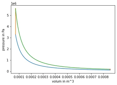

pv diagram of otto cycle

conclusion

using python pv diagram is ploted and state poins are calculted and efficiency also found

efficincy of otto cycle is calculated as 62.98%