Week 2 Air standard Cycle

Aim : To create a PV diagram of an otto cycle and to find its thermal efficiency using python.

Objective :

• To create a PV Diagram of an Otto Cycle using PYTHON.
• To determine the Thermal Efficiency of the Otto Cycle.

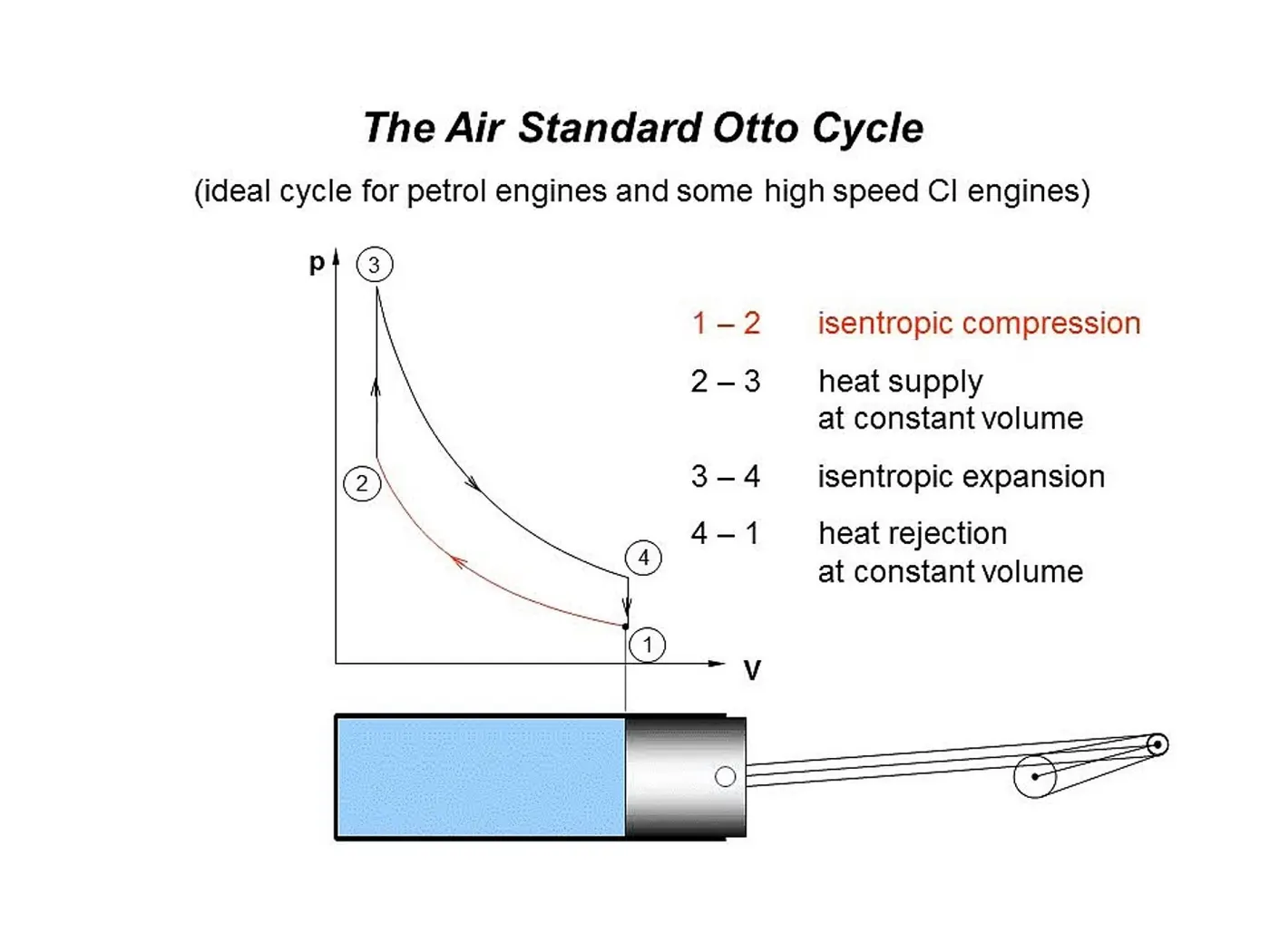
Theory : The otto cycle or air standard cycle consists of four cycles they are

• process 1-2 : Isentropic compression.
• process 2-3 : Constant volume heat addition.
• process 3-4 : Isentropic expanssion.
• process 4-1 : Constant volume heat rejection.

Engine geometric parameters :

• Bore
• Stroke
• Connecting rod length
• Compression ratio.

Explanation :

• Swept volume = volume of the cylinder.(pi/4*d^2*l).
• Clearance volume = swept volume/cr-1.
• v1 = swept volume + clearance volume.
• v2 = clearance volume.
• here pv/t = constant.

Input values :

Engine geometric parameters :

• bore = 0.1
• stroke = 0.1
• con_rod = 0.15
• cr = 8
• γ=γ=1.4 (for air).

CODE IN PYTHON :

# Otto cycle simulator
import math
import matplotlib.pyplot as plt

def Engine_kinematics(bore, stroke, con_rod, cr, start_crank, end_crank):

    # Engine kimenatics
    
    # Geometrical parameters
    a = stroke/2
    R = con_rod/a

    # Volume parameters 
    v_s = (math.pi/4)*pow(bore,2)*stroke
    v_c = v_s/(cr-1)

    sc = math.radians(start_crank)
    ec = math.radians(end_crank)

    num_values = 50

    dtheta = (ec - sc)/(num_values - 1)

    v = []

    for i in range(0,num_values):
        theta = sc + i*dtheta
        term1 = 0.5*(cr-1)
        term2 = R + 1 - math.cos(theta)
        term3 = pow(R,2) - pow(math.sin(theta),2)
        term3 = pow(term3, 0.5)
        v.append((1 + term1*(term2 - term3))*v_c)

    return v        

# inputs
p1 = 101325
t1 = 500
gamma = 1.4
t3 = 2300

# Geometric parameters
bore = 0.1
stroke = 0.1
con_rod = 0.15
cr = 8

# Volume computation
v_s = (math.pi/4)*pow(bore,2)*stroke
v_c = v_s/(cr-1)
v1 = v_c + v_s

# State point 2
v2 = v_c

# p2v2^gamma = p1v1^gamma
p2 = p1*pow(v1,gamma)/pow(v2,gamma)

# p2v2/t2 = p1v1/t1 | rhs = p1v1/t1 | rhs = p2v2/t2 | t2 = p2v2/rhs
rhs = p1*v1/t1
t2 = p2*v2/rhs
v_compression = Engine_kinematics(bore,stroke, con_rod, cr, 180, 0)

constant = p1*pow(v1,gamma)

p_compression = []

for v in v_compression:
    p_compression.append(constant/pow(v, gamma))

# state point 3
v3 = v2

# p3v3/t3 = p2v2/t2 | rhs = p2v2/t2 | p3 = rhs*t3/v3
rhs = p2*v2/t2
p3 = rhs*t3/v3

v_expansion = Engine_kinematics(bore,stroke, con_rod, cr, 0, 180)

constant = p3*pow(v3,gamma)

p_expansion = []

for v in v_expansion:
    p_expansion.append(constant/pow(v, gamma))

# State point 4 
v4 = v1

# p4v4^gamma = p3v3^gamma
p4 = p3*pow(v3,gamma)/pow(v4,gamma)

# p4v4/t4 = rhs
t4 = p4*v4/rhs

plt.plot([v2,v3],[p2,p3])
plt.plot(v_compression, p_compression)
plt.plot(v_expansion, p_expansion)
plt.plot([v4,v1],[p4,p1])
plt.xlabel('Volume(m^3)')
plt.ylabel('Pressure(pa)')
plt.title('P-V diagram of an Otto cycle')
plt.show()

# Thermal efficiency
n = 1 - (pow(cr,(1-gamma)))
print(n)

Code explanation :

• Initially, writing a function program where a specified function is mentioned covering all the parameters and the variables.
• Equations and the respective variables are defined.
• Further, we write the main program starting with mentioning state variables and engine geometric parameters.
• Thereafter, we specify the equations being used during the processes starting from state 1 to state 4.
• The function program is called for the states 1-2 and 3-4 because they constitute a different process, i.e. isentropic process.
• After providing the equations, plotting of PV diagram is done followed by the calculation of Thermal Efficiency.

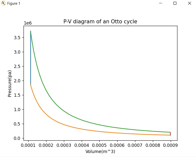
Result of P-V Diagram :

Thermal effiency of otto cycle :

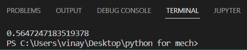
Therefore thermal effiency of otto cycle in percentage = 56.47 %.

Conclusion :

The PV Diagram has been plotted using the process equations and the thermal efficiency has been calculated. It can be observed that the efficiency varies inversely with the compression ratio.