Week 2 Air standard Cycle

Aim

Write code that can solve an otto cycle and make plots for it. The code should also output the thermal efficiency of the engine.

Governing equations

An Otto cycle is an idealized thermodynamic cycle that describes the functioning of a typical spark ignition piston engine. It is the thermodynamic cycle most commonly found in automobile engines.

The Otto cycle is a description of what happens to a mass of gas as it is subjected to changes of pressure, temperature, volume, the addition of heat, and removal of heat. The mass of gas that is subjected to those changes is called the system. The system, in this case, is defined to be the fluid (gas) within the cylinder. By describing the changes that take place within the system, it will also describe in the inverse, the system's effect on the environment. In the case of the Otto cycle, the effect will be to produce enough net work from the system so as to propel an automobile and its occupants in the environment.

The Otto cycle is constructed from:

• Top and bottom of the loop: a pair of quasi-parallel and isentropic processes (frictionless, adiabatic reversible).
• Left and right sides of the loop: a pair of parallel isochoric processes (constant volume).

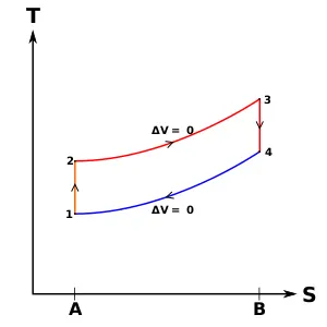
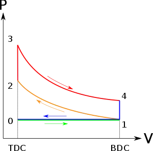
In the above diagrams:

p = pressure

V = Volume

T = temperature

s = Entropy

`V_c` = Clearance volume

`V_s` = Stroke Volume

Processes

The processes are described by:

• Process 0–1 a mass of air is drawn into piston/cylinder arrangement at constant pressure.
• Process 1–2 is an adiabatic (isentropic) compression of the charge as the piston moves from the bottom dead center (BDC) to top dead center (TDC).

Heat Supplied = m`C_v`(`T_3`-`T_2` ; where m = mass and `C_v`= Specific heat at constant volume

• Process 2–3 is a constant-volume heat transfer to the working gas from an external source while the piston is at top dead center. This process is intended to represent the ignition of the fuel-air mixture and the subsequent rapid burning.
• Process 3–4 is an adiabatic (isentropic) expansion (power stroke).
• Process 4–1 completes the cycle by a constant-volume process in which heat is rejected from the air while the piston is at bottom dead center.

Heat Rejected = m`C_v`(`T_4-T_1`)

• Process 1–0 the mass of air is released to the atmosphere in a constant pressure process.

Thermal efficiency of air standard cycle (or Otto Cycle),

`eta_(th) = ( Heat Supplied - Heat Rejected)/(Heat Supplied)`

`eta_(th) = 1 - (T_4-T_1)/(T_3-T_2)`

Process 1-2 and 3-4 are isentropic and hence,

`T_4(V_1)^(gamma-1) = T_3(V_2)^(gamma-1) ; T_1V_1^(gamma - 1) = T_2V_2^(gamma-1)`

Swept volume, `V_s = (pi*b^2*stroke)/4`

Clearance volume, `V_c = V_s/(cr-1)

The Otto cycle consists of isentropic compression, heat addition at constant volume, isentropic expansion, and rejection of heat at constant volume. In the case of a four-stroke Otto cycle, technically there are two additional processes: one for the exhaust of waste heat and combustion products at constant pressure (isobaric), and one for the intake of cool oxygen-rich air also at constant pressure; however, these are often omitted in a simplified analysis. Even though those two processes are critical to the functioning of a real engine, wherein the details of heat transfer and combustion chemistry are relevant, for the simplified analysis of the thermodynamic cycle, it is more convenient to assume that all of the waste-heat is removed during a single volume change.

Given:

bore = 0.8

stroke = 0.2

connecting rod length = 0.15

compression ratio = 12

p1 = 101325

gamma = 1.4

t1 = 550

t3 = 2800

Python code

'''
Program to calculate different state variables in an otto cycle and to calculate its thermal efficiency
'''

import math
import matplotlib.pyplot as plt

def engine_kinematics(bore,stroke,con_rod,cr,start_crank,end_crank):
    
    # Geometric parameters
    a = stroke/2
    R = con_rod/a

    # Volume parameters
    V_s = math.pi*(1/4)*pow(bore,2)*stroke
    V_c = V_s/(cr-1)

    sc = math.radians(start_crank)
    ec = math.radians(end_crank)

    num_values = 100
    dtheta = (ec-sc)/(num_values)

    V = []

    for i in range(0,num_values):
        theta = sc + i*dtheta
        term1 = 0.5*(cr-1)
        term2 = R +1 - math.cos(theta)
        term3 = pow(R,2) - pow(math.sin(theta),2)
        term3 = pow(term3,0.5)

        V.append((1+term1*(term2-term3))*V_c)
    
    return V

# Inputs
p1 = 101325
t1 = 550
gamma = 1.4
t3 = 2800

# Geometric parameters
bore = 0.8
stroke = 0.2
con_rod = 0.15
cr = 12

# Computing the volume
v_s = (math.pi/4)*pow(bore,2)*stroke
v_c = v_s/(cr-1)
v1 = v_c + v_s


# State variables at point 2
v2 = v_c

# p2v2^gamma = p1v1^gamma
p2 =p1*pow(v1,gamma)/pow(v2,gamma)

# p2v2/t2 = p1v1/t1 | rhs = p1v1/t1 | p2v2/t2 = rhs | t2 = p2v2/rhs
rhs = p1*v1/t1
t2 = p2*v2/rhs
V_compression = engine_kinematics(bore,stroke,con_rod,cr,180,0)

constant = p1*pow(v1,gamma)

P_compression = []

for v in V_compression:
    P_compression.append(constant/pow(v,gamma))


# State variables at point 3
v3 = v2

#p3v3/t3 = p2v2/t2 | rhs = p2v2/t2 | p3 = rhs*t3/v3
rhs = p2*v2/t2
p3 = rhs*t3/v3

V_expansion = engine_kinematics(bore,stroke,con_rod,cr,0,180)

constant = p3*pow(v3,gamma)

P_expansion = []

for v in V_expansion:
    P_expansion.append(constant/pow(v,gamma))


# State variables at point 4
v4 = v1

# p4v4^gamma = p3v3^gamma
p4 = p3*pow(v3,gamma)/pow(v4,gamma)

# p4v4/t4 = rhs
t4 = p4*v4/rhs

# Calculating the thermal efficiency

thermal_eff = (1 - (1/pow((cr),(gamma-1))))*100
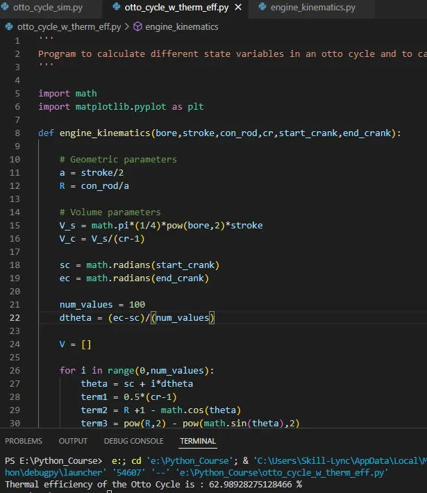
print('Thermal efficiency of the Otto Cycle is :',thermal_eff,'%')

# Plotting the state points
plt.plot([v2,v3],[p2,p3])
plt.plot(V_compression,P_compression)
plt.plot(V_expansion,P_expansion)
plt.plot([v4,v1],[p4,p1])
plt.xlabel('Volume (m^3)')
plt.ylabel('Pressure (Pa)')
plt.title('P-V diagram of an Otto Cycle')
plt.grid()
plt.show()

Code explanation:

1. All known geometric parameters and state variables are defined
2. The formula for clearance volume and swept volume was provided.
3. For process 1-2 and 3-4, all state variables were calculated using Isentropic formulae.
4. Now, we obtained all four points but we need to define the changes in volume.
5. For this, a function engine_kinematics was defined which calculates the swept volume for isentropic processes for each value of angle covered.
6. Bore, stroke, length of connecting rod, compression ratio, and swept volume are given as arguments.
7. The thermal efficiency formula is also defined before plotting.
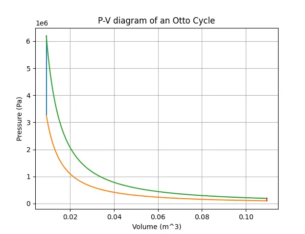
8. A P-V diagram is obtained with the help of plot command.

Errors faced

Faced errors due to typos in certain instances, resolved them by correcting the typos.

Output

The program outputs the efficiency of the Otto cycle and plot p-V diagram. We can see that for heat addition and heat rejection process, the volume is constant and for the isentropic processes, the graph follows an isentropic path.

Conclusion

The thermal efficiency was calculated with the help of a python program and a p-V diagram was plotted as well.

The thermal efficiency of the Otto Cycle was found to be 62.98%.