Week 2 Air standard Cycle
Course: Python for Mechanical Engineers
Challenge: Air Standard Cycle
Submitted By: Amanpreet Singh Whan
1 Aim:
The aim of the week 2 challenge is to write code that can solve an otto cycle and make plots for it.
2 Theory and Governing Equations:
The Otto Cycle is named after Nikolaus Otto (1832–1891, German) who is credited as the first creator of a petroleum fuel-based internal combustion engine operating under a four-stroke cycle. Otto’s engine work during the eve of the industrial revolution was a critical development leading to the dawn of the automotive industry in the late 19th century. The Otto Cycle involves four engine strokes. A stroke is defined as a process in which the cylinder’s piston moves up to the top of the engine or down to the bottom of the engine. The cycle begins with the intake stroke in which fresh reactants (fuel and air) are drawn into the engine’s cylinder by a downward-expanding piston motion. The second stroke is compression in which the piston moves from the bottom to the top of the engine thereby reducing the volume of the fuel and air. Compressing the reactants before burning them allows for greater work and power to be extracted from the following combustion process. When the piston is near the top of its stroke combustion begins and expansion of the burned gases continues into the expansion stroke. The last of the four strokes is the exhaust stroke in which the burned products of combustion are pushed out of the engine to make space for the next cycle’s intake stroke. The Otto cycle is the ideal cycle for spark-ignition (SI) engines. This cycle was presented in the late 19th century after Nikolaus Otto demonstrated the four-stroke SI engine successfully [1]. Description of the processes is given as follows:
- Process 1-2: isentropic compression of the working fluid occurs as the piston moves from the bottom dead center (BDC) to the top dead center (TDC).
- Process 2-3: here, with the SI, a rapid burning occurs inside the piston; therefore, the heat addition takes place at a constant volume.
- Process 3-4: in this process, the working fluid expands isentropically and produces useful work for the cycle.
- Process 4-1: heat removal at constant volume. In practical applications, the heat is removed by expelling the exhaust gas into the atmosphere.
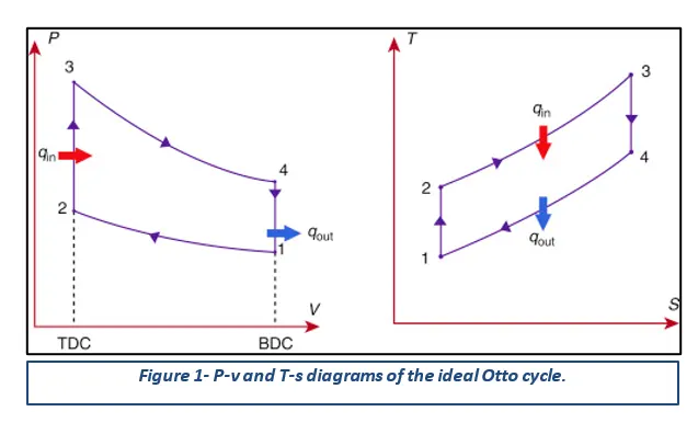
3 Objectives:
The objectives of the week 2 challenges are as follows:
- Written program should plot a PV diagram of the Otto Cycle.
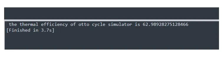
- Also, write a code to calculate the thermal efficiency of the Otto Cycle.
4 Body of the Content:
Python is an interpreted, object-oriented, high-level programming language with dynamic semantics. Its high-level built-in data structures, combined with dynamic typing and dynamic binding, make it very attractive for Rapid Application Development, as well as for use as a scripting or glue language to connect existing components. Python's simple, easy-to-learn syntax emphasizes readability and therefore reduces the cost of program maintenance. Python supports modules and packages, which encourages program modularity and code reuse.
The formula to calculate volume is as follows:

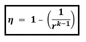
The formula used to calculate thermal efficiency is as follows:
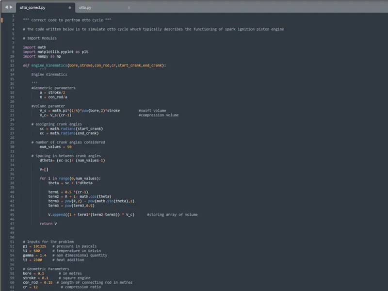
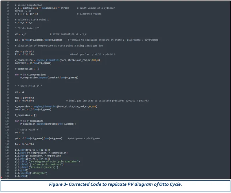
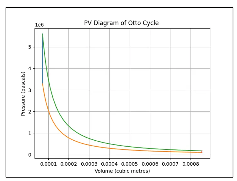
The python code was written to fulfill the requirements of the Week 2 challenge and is attached in the following figures. In addition, the PV plot obtained from the written code is attached as well.
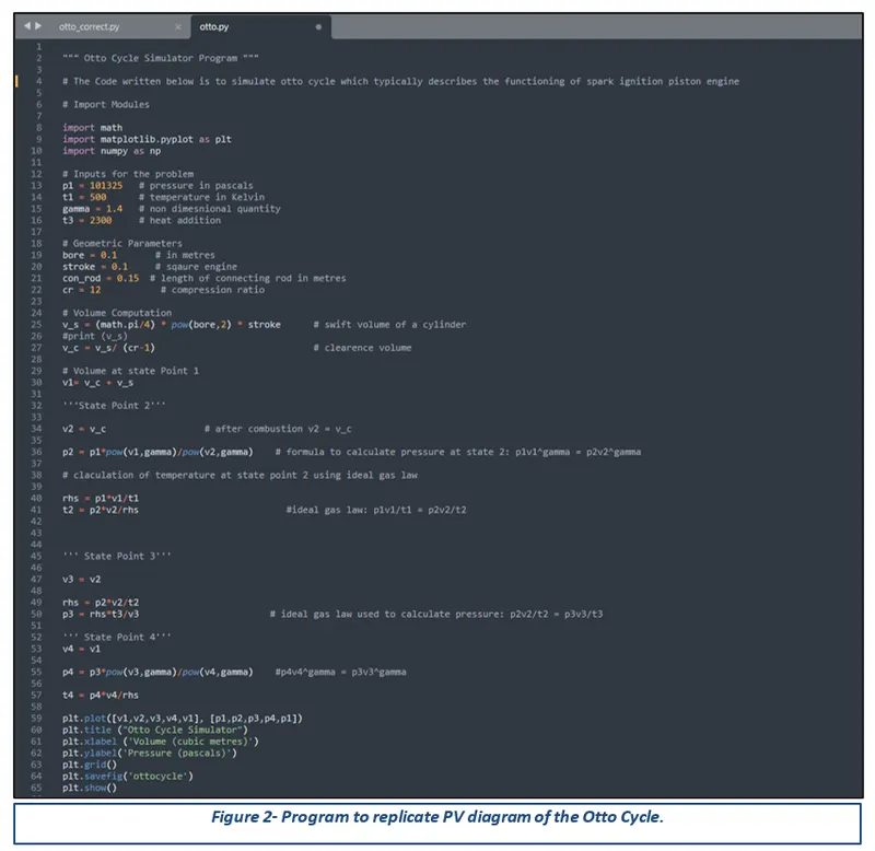
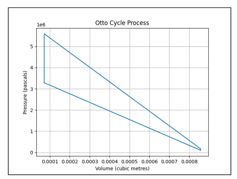
The code was written to solve an otto cycle using python resulting in sound and acceptable values. However, from the plotted PV diagram, it was found that the curve follows a linear pattern instead of a parabolic pattern. Therefore, the modified code/ program that produces accurate and precise results is presented in the following figure.
5 Conclusion:
In conclusion, the main aim of the week 2 challenge is to write a python program that can solve an otto cycle and make plots for it. In addition, write a program to calculate the thermal efficiency for the same.
In total, two python programs were written to replicate the PV diagram of the Otto Cycle. The first program plotted PV curves with a linear pattern and therefore the code was adjusted and modified to approximately replicate the PV curves with a parabolic pattern. The thermal efficiency calculated using the python was found to be 62.98 %
6 Appendix:
Program - 1
""" Otto Cycle Simulator Program """

# The Code written below is to simulate otto cycle which typically describes the functioning of spark ignition piston engine

# Import Modules

import math
import matplotlib.pyplot as plt
import numpy as np

# Inputs for the problem
p1 = 101325   # pressure in pascals
t1 = 500      # temperature in Kelvin
gamma = 1.4   # non dimesnional quantity
t3 = 2300     # heat addition

# Geometric Parameters
bore = 0.1       # in metres
stroke = 0.1     # sqaure engine
con_rod = 0.15  # length of connecting rod in metres
cr = 12           # compression ratio

# Volume Computation
v_s = (math.pi/4) * pow(bore,2) * stroke      # swift volume of a cylinder
#print (v_s)
v_c = v_s/ (cr-1)                             # clearence volume

# Volume at state Point 1
v1= v_c + v_s

'''State Point 2'''

v2 = v_c                  # after combustion v2 = v_c

p2 = p1*pow(v1,gamma)/pow(v2,gamma)    # formula to calculate pressure at state 2: p1v1^gamma = p2v2^gamma

# claculation of temperature at state point 2 using ideal gas law

rhs = p1*v1/t1
t2 = p2*v2/rhs                           #ideal gas law: p1v1/t1 = p2v2/t2


''' State Point 3'''

v3 = v2

rhs = p2*v2/t2
p3 = rhs*t3/v3                        # ideal gas law used to calculate pressure: p2v2/t2 = p3v3/t3

''' State Point 4'''
v4 = v1

p4 = p3*pow(v3,gamma)/pow(v4,gamma)    #p4v4^gamma = p3v3^gamma

t4 = p4*v4/rhs

plt.plot([v1,v2,v3,v4,v1], [p1,p2,p3,p4,p1])
plt.title ("Otto Cycle Process")
plt.xlabel ('Volume (cubic metres)')
plt.ylabel('Pressure (pascals)')
plt.grid()
plt.savefig('ottocycle')
plt.show()
Modified and Corrected Program - 2
""" Correct Code to perfrom Otto Cycle """

# The Code written below is to simulate otto cycle whuch typically describes the functioning of spark ignition piston engine

# Import Modules

import math
import matplotlib.pyplot as plt
import numpy as np

def engine_kinematics(bore,stroke,con_rod,cr,start_crank,end_crank):
		'''
	Engine Kinematics

	'''
	#Geometric parameters
		a = stroke/2
		R = con_rod/a

	#Volume paramter
		V_s = math.pi*(1/4)*pow(bore,2)*stroke         #swift volume
		V_c= V_s/(cr-1)                                #compression volume

	# assigning crank angles
		sc = math.radians(start_crank)
		ec = math.radians(end_crank)

	# number of crank angles considered
		num_values = 50

	# Spacing in between crank angles
		dtheta= (ec-sc)/ (num_values-1)

		V=[]

		for i in range(0,num_values):
			theta = sc + i*dtheta

			term1 = 0.5 *(cr-1)
			term2 = R + 1- math.cos(theta)
			term3 = pow(R,2) - pow(math.sin(theta),2)
			term3 = pow(term3,0.5)

			V.append((1 + term1*(term2-term3)) * V_c)  #storing array of volume

		return V


# Inputs for the problem
p1 = 101325   # pressure in pascals
t1 = 500      # temperature in Kelvin
gamma = 1.4   # non dimesnional quantity
t3 = 2300     # heat addition

# Geometric Parameters
bore = 0.1       # in metres
stroke = 0.1     # sqaure engine
con_rod = 0.15  # length of connecting rod in metres
cr = 12           # compression ratio

# Volume Computation
v_s = (math.pi/4) * pow(bore,2) * stroke      # swift volume of a cylinder
#print (v_s)
v_c = v_s/ (cr-1)                             # clearence volume

# Volume at state Point 1
v1= v_c + v_s

'''State Point 2'''

v2 = v_c                  # after combustion v2 = v_c

p2 = p1*pow(v1,gamma)/pow(v2,gamma)    # formula to calculate pressure at state 2: p1v1^gamma = p2v2^gamma

# claculation of temperature at state point 2 using ideal gas law

rhs = p1*v1/t1
t2 = p2*v2/rhs                           #ideal gas law: p1v1/t1 = p2v2/t2

V_compression = engine_kinematics(bore,stroke,con_rod,cr,180,0)
constant = p1*pow(v1,gamma)

P_compression = []

for v in V_compression:
	P_compression.append(constant/pow(v,gamma))


''' State Point 3'''

v3 = v2

rhs = p2*v2/t2
p3 = rhs*t3/v3                        # ideal gas law used to calculate pressure: p2v2/t2 = p3v3/t3

V_expansion = engine_kinematics(bore,stroke,con_rod,cr,0,180)
constant = p3*pow(v3,gamma)

P_expansion = []

for v in V_expansion:
	P_expansion.append(constant/pow(v,gamma))

''' State Point 4'''
v4 = v1

p4 = p3*pow(v3,gamma)/pow(v4,gamma)    #p4v4^gamma = p3v3^gamma

t4 = p4*v4/rhs

plt.plot([v2,v3], [p2,p3])
plt.plot (V_compression, P_compression)
plt.plot(V_expansion, P_expansion)
plt.plot([v4,v1], [p4,p1])
plt.title ("PV Diagram of Otto Cycle ")
plt.xlabel ('Volume (cubic metres)')
plt.ylabel('Pressure (pascals)')
plt.grid()
plt.savefig('otto cycle')
plt.show()


''' code to calculate Thermal Efficiency of Otto Cycle Simulator'''

Thermal_efficiency = 1 - (1/pow(cr,(gamma-1)))
Thermal_efficiency_percentage = Thermal_efficiency * 100
print (f" the thermal efficiency of otto cycle simulator is {Thermal_efficiency_percentage}")