Week 2 Air standard Cycle

Aim:

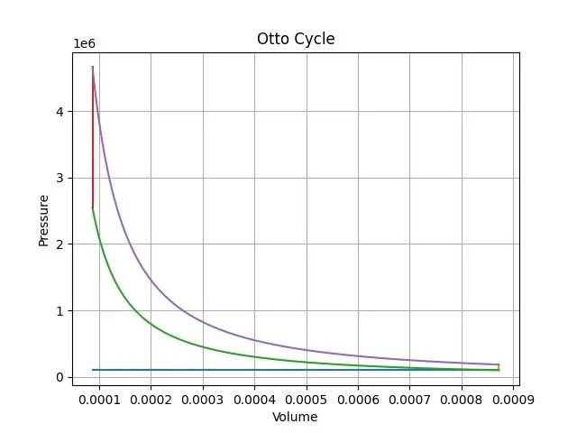
To plot PV diagram of an Otto cycle using python software

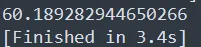
To estimate the overall efficiency

Otto Cycle:

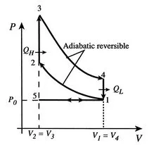
The Otto cycle is a set of processes used by spark-ignition internal combustion engines. These engines a) intake a mixture of fuel and air, b) compress it, c) heat addition to the mixture, d) expand the combustion products, and then e) eject the combustion products and replace them with a new charge of fuel and air. The different processes are shown in

1. Intake stroke, gasoline vapor, and air is drawn into the engine ( 5 to 1 ).
2. Compression stroke ie (isentropic compression) ( 1 to 2).
3. Combustion essentially at constant volume ( 2 to 3).
4. Power stroke: expansion (isentropic expansion) ( 3 to 4 ).
5. Valve exhaust: valve opens, gas escapes.
6. ( 4 to 1 ) Model: heat rejection at constant volume.
7. Exhaust stroke, the piston pushes remaining combustion products out of the chamber ( 1 to 5).

Formulae Used :

Swept volume, clearance volume calculation

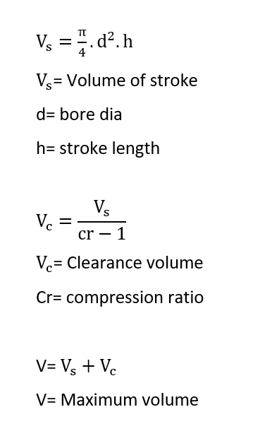
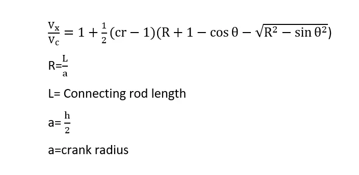
Relationship between Volume of the cylinder and the crank angle

Otto cycle Efficiency

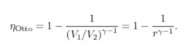
r= compression ratio

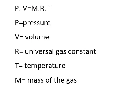
Ideal gas equation

Procedures

• Library functions such as matplotlib, math is used to plot and do mathematical calculations.
• The value of the pressure, volume, and temperature are found at (1,2,3,4)(state) by using Ideal gas law.
• The state of the properties at each point(between 1 and 2) is found by using the volume, crank angle, and relationship formula.
• In order to achieve this function in python is used, A function is a block of code that only runs when it is called. Users can pass data, known as parameters, into a function. A function can return data as a result.

The syntax for defining a function

def my_function():
print("Hello from a function")

def is used to define a function

my_function is the name of the function

The return statement is used to send the processed data whenever the function is called

Function

# Function for calculating compression expansion volume
def enginekinematics(bore,stroke,con_rod,cr,start_angle,end_angle):
	# Geometric properties
	a=stroke/2   # crank radius
	R=con_rod/a 
	# Start and end angle definition
	sa=math.radians(start_angle)
	ea=math.radians(end_angle)
	dtheta=(ea-sa)/(number_angle-1)
	V=[]
	for i in range (0,number_angle):
		theta=sa+(i*dtheta)
		term1=0.5*(cr-1)
		term2= R+1-math.cos(theta)
		term3=pow(R,2)-pow(math.sin(theta),2)
		term3=pow(term3,0.5)
		V.append((1+(term1*(term2-term3)))*v_clearance)
	return V

Program:

''' Otto cycle
'''
import matplotlib.pyplot as plt 
import math  

# geometric parameters
bore=0.1
stroke=0.1
con_rod=0.15
cr=10
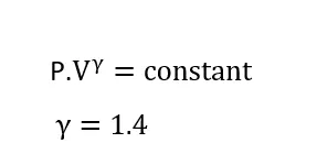
gamma=1.4

# Volume computation
v_stroke=(math.pi/4)*pow(bore,2)*stroke
v_clearance=(v_stroke/(cr-1))

# Angle properties
number_angle=1000

# Function for calculating compression expansion volume
def enginekinematics(bore,stroke,con_rod,cr,start_angle,end_angle):
	# Geometric properties
	a=stroke/2   # crank radius
	R=con_rod/a 
	# Start and end angle definition
	sa=math.radians(start_angle)
	ea=math.radians(end_angle)
	dtheta=(ea-sa)/(number_angle-1)
	V=[]
	for i in range (0,number_angle):
		theta=sa+(i*dtheta)
		term1=0.5*(cr-1)
		term2= R+1-math.cos(theta)
		term3=pow(R,2)-pow(math.sin(theta),2)
		term3=pow(term3,0.5)
		V.append((1+(term1*(term2-term3)))*v_clearance)
	return V

# PV diagram parameters
# variables at state 1
v1=v_stroke+v_clearance
p1=101325
t1=500
constant=(p1*pow(v1,gamma))
v_compression=enginekinematics(bore,stroke,con_rod,cr,180,0)
pc=[]
for vc in v_compression:
	pc.append(constant/pow(vc,gamma))
p_compression=pc


# variables at state 2
v2=v_clearance
p2=(p1*pow(v1,gamma))/(pow(v2,gamma))
t2=(p2*v2*t1)/(p1*v1) 


# variables at state 3
v3=v2
t3=2300
p3=(p2*v2*t3)/(v3*t2)
constant=(p3*pow(v3,gamma))
v_expansion=enginekinematics(bore,stroke,con_rod,cr,0,180)
pe=[]
for ve in v_expansion:
	pe.append(constant/pow(ve,gamma))
p_expansion=pe 
print(p_expansion)

# variables at state 4
v4=v1
p4=(p3*pow(v3,gamma))/(pow(v4,gamma))
t4=(p4*v4*t1)/(p1*v1)

# Efficiency
efterm=1/(pow(cr,(gamma-1)))
Efficiency=(1-efterm)*100
print(Efficiency)



# plotting the curve
p0=101325
plt.plot([v2,v4],[p1,p0])
plt.plot([v1,v4],[p1,p4])
plt.plot(v_compression,p_compression)
plt.plot([v2,v3],[p2,p3])
plt.plot(v_expansion,p_expansion)
plt.title("Otto Cycle")
plt.xlabel("Volume")
plt.ylabel("Pressure")
plt.grid()
plt.show()

Output

PV diagram

Thermal Efficiency

The thermal efficiency is found to be

Conclusion

• Area of the otto cycle decreases as the compression ratio increases.
• The efficiency of the cycle increases with an increase in compression ratio