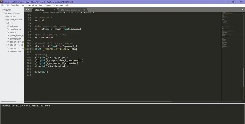
Week 2 Air standard Cycle

Aim : To write a code for otto cycle and plot a PV graph as well as find the efficiency of the engine

Theory :

An Otto cycle is an idealized therodynamic cycle that describes the functioning of a typical spark ignition piston engine. It is the thermodynamic cycle most commonly found in automobile engines.

import math       #for mathematical functions
import matplotlib.pyplot as plt

def engine_kinematics(bore,stroke,con_rod,cr,start_crank,end_crank):   #function is made so that we get a program that gives us a array of volume for the crank angle that corresponds to compression and expansion
# we can use this to calculate pressures corresponding to the values
	# engine kinematics 

	import math
	#geometric parameters
	bore=0.10
	stroke = 0.1
	con_rod=0.15   #connecting rod length
	cr=12  #compression ratio
	a = stroke/2  #crank pin radius
	R = con_rod/a

	#volume parameters
	V_s = (math.pi/4)*pow(bore,2)*stroke      #swept volume
	V_c = V_s/(cr-1)   #clearance volume

	sc = math.radians(start_crank)
	ec = math.radians(end_crank)

	num_values = 50

	dtheta = (ec-sc)/(num_values-1)

	V=[]

	for i in range(0,num_values):
		theta = sc+i*dtheta
		term1 = 0.5*(cr-1)
		term2 = R+1-math.cos(theta)
		term3= pow(R,2)-pow(math.sin(theta),2)
		term3 = pow(term3,0.5)

		V.append((1 + term1*(term2-term3))*V_c)   #volume
	return V

	

  

#inputs
p1 = 101325          #pressure at state one as 1atm = 101325 pa
t1 = 500             #temperature at state one 
gamma = 1.4
t3 = 2300
#geometric parameters
bore = 0.1
stroke = 0.1
con_rod = 0.15       #length of connecting rod
cr = 12             #compression ratio 

#volume computation
v_s = (math.pi/4)*pow(bore,2)*stroke      #swept volume
v_c = v_s/(cr-1)                          #compression volume
v1 = v_s + v_c                             #volume at state one

#state point 2
v2 = v_c  #after compression,volume uncer compression is equal to clearance 

#pressure p2v2^gamma = p1v1^gamma
p2 = p1*pow(v1,gamma)/pow(v2,gamma)

# p2v2/t2 = p1v1/t1 |rhs = p1v1/t1 | p2v2/t2=rhs | t2=p2v2/rhs
rhs = p1*v1/t1
t2 = p2*v2/rhs

V_compression= engine_kinematics(bore,stroke,con_rod,cr,180,0)   #function is made so that we get a program that gives us a array of volume for the crank angle that corresponds to compression and expansion
constant = p1*pow(v1,gamma)

P_compression =[]
for v in  V_compression:
	P_compression.append(constant/pow(v,gamma))


#state point 3(right after combustion)
v3 = v2

#p3v3/t3=p2v2/t2 | rhs = p2v2/t2 | p3=rhs*t3/v3
rhs = p2*v2/t2
p3 = rhs*t3/v3

V_expansion= engine_kinematics(bore,stroke,con_rod,cr,0,180)   #function is made so that we get a program that gives us a array of volume for the crank angle that corresponds to compression and expansion
constant = p3*pow(v3,gamma)

P_expansion =[]
for v in  V_expansion:
	P_expansion.append(constant/pow(v,gamma))

#statepoint 4
v4 = v1

#p4v4^gamma = p3v3^gamma
p4 = p3*pow(v3,gamma)/pow(v4,gamma)

#p4v4/t4 = p3v3/t3 = rhs 
t4 = p4*v4/rhs

#thermal efficiency of engine
eta = 1 - (1/pow(v1/v2,gamma-1))
print ('thermal efficiency',eta)

#plotting
plt.plot([v2,v3],[p2,p3])
plt.plot(V_compression,P_compression)
plt.plot(V_expansion,P_expansion)
plt.plot([v4,v1],[p4,p1])

plt.show()

Result :

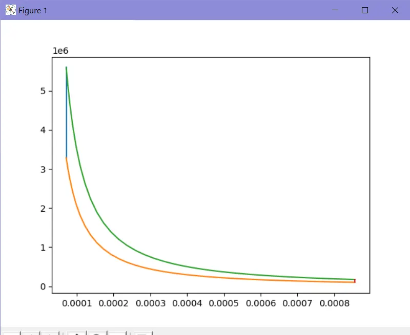
In this graph, the orange curve shows an adiabatic compression. The straight blue line shows heat transfer at a constant volume , the green curve represents adiabatic expansion and in the end the red straight line denotes the constant volume where heat is rejected .

Output :