Week 2 Air standard Cycle

Aim: To write a code for the Otto cycle and extract the p-v plot and

the efficiency of Otto cycle using python script.

Procedure: 1. Open a sublime text editor and save the file as otto cycle.py

and then import all useful library like math and matplotlib.

2. Now define the engine parameters using the 'def' command and calculate the

The volume of the cylinder and append the volume up to 50 values.

Here the volume formula is split into three terms and then calculated.

3. Now define the input parameters like pressure, temperature and

the air constant gamma and also define the compression ratio, stroke

length, bore diameter and connecting rod length.

4. After defining all input parameters now start calculating the

pressure, volume and temperature and write the code in the format of code.

5. To calculate pressure and volume at the compression and

expansion process write a 'for' loop function and append the

pressure with respect to volume at the compression and expansion.

6. Now write the command to calculate the thermal efficiency of this cycle.

7. Now write the commands to plot the p-v diagram and mention legends at the x-axis and y-axis.

8. Now save the file again and run the whole script and we get the plot and thermal efficiency.

CODE-

#otto cycle simulator
#Engine kinematics

#import library
import math
import matplotlib.pyplot as plt 

def engine_kinematics(bore,stroke,conn_rod,c_r,start_crank,end_crank):

    #Engine parameters
	a = stroke/2
	R = conn_rod/a
	c_r = 10

	#Volume Calculations
	v_s = (math.pi/4)*pow(bore,2)*stroke
	v_c = v_s/(c_r-1)

	#strating crank angle and ending crank angle
	sc = math.radians(start_crank)
	ec = math.radians(end_crank)

	num_values = 50
	dtheta = (ec-sc)/(num_values-1)

	V =[]

	#write the 'for' loop command to calculate volume
	for i in range(0,num_values-1):

		theta = sc + i*dtheta

		term1 = 0.5*(c_r-1)
		term2 = R + 1-math.cos(theta)
		term3 = pow(R,2) - pow(math.sin(theta),2)
		term3 = pow(term3,0.5)

		V.append((1 + term1*(term2 -term3))*v_c)

	return V
#intial inputs of pressure,temperature and value of isentropic expansion factor gamma
p1 = 101325
t1 = 500
gamma = 1.4
t3 = 2300

#engine parameters 
bore = 0.15
stroke = 0.2
conn_rod = 0.8
c_r = 10


#volume calculations for swept volume and compression volume
v_s = (math.pi/4)*pow(bore,2)*stroke
v_c = v_s/(c_r-1)
v1 = v_c + v_s

#constant volume process
v2 = v_c
#from isentropic process p2v2^gamma = p1v1^gamma
p2 = p1*pow(v1,gamma)/pow(v2,gamma)

#to find temperature value at 2nd use ideal gas equation
rhs = p1*v1/t1
t2 = p2*v2/rhs
V_compression = engine_kinematics(bore,stroke,conn_rod,c_r,180,0)

constant = p1*pow(v1,gamma)

P_compression = []

for v in V_compression:
	P_compression.append(constant/pow(v,gamma))

#at stage 3
v3 = v2
rhs_1 = p2*v2/t2
p3 = t3*rhs_1/v3

V_expansion = engine_kinematics(bore,stroke,conn_rod,c_r,0,180)

constant = p3*pow(v3,gamma)

P_expansion = []

for v in V_expansion:
	P_expansion.append(constant/pow(v,gamma))


#at stage 4
v4 = v1
p4 = p3*pow(v3,gamma)/(pow(v4,gamma))

#final temperature
rhs_2 = p3*v3/t3 
t4 = p4*v4/rhs_2

#calcuate efficiency of otto cycle = n
n = 1 - (1/pow((c_r),(gamma -1)))
print(n)


#write the commands for plotting

plt.plot(V_compression,P_compression)
plt.plot([v2,v3,],[p2,p3])
plt.plot(V_expansion,P_expansion)
plt.plot([v4,v1],[p4,p1])
plt.ylim([-500000,8000000])
plt.xlim([0,0.005])
plt.ylabel('Pressure')
plt.xlabel('Volume')
plt.title('Otto Cycle')
plt.grid()
plt.show()

GRAPH-

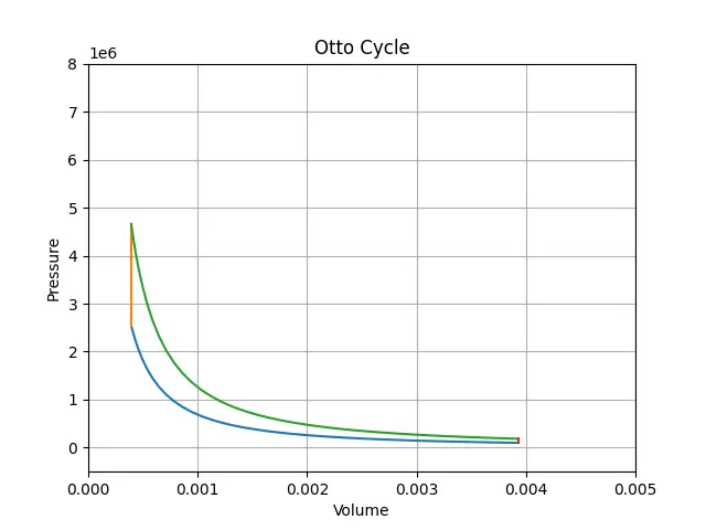
We can see the result in the image below

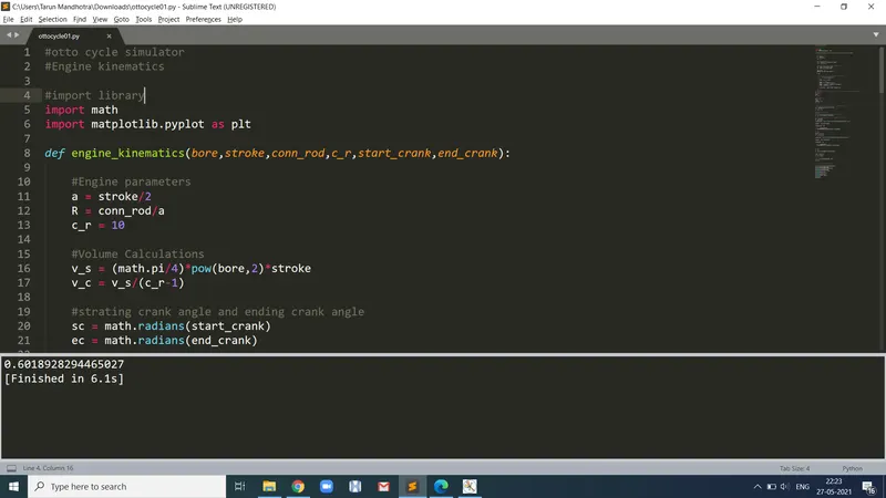
The thermal efficiency of this cycle is 60% and the p-v diagram of the otto cycle is plotted perfectly.

RESULT -Here we achieve the results as per the given instruction.