Week 2 Air standard Cycle

AIM:

To generate a PV diagram of an Air Standard Cycle (Otto Cycle),

and also to calculate the thermal efficiency of the engine through a python code.

Process in the otto cycle

The thermodynamic analysis of the actual four-stroke or two-stroke cycles described is not a simple task.

However, the analysis can be simplified significantly if the air-standard assumptions are utilized.

The resulting cycle, which closely resembles the actual operating conditions, is the ideal Otto cycle.

It consists of four internally reversible processes:

1-2 Isentropic compression

2-3 constant-volume heat addition

3-4 Isentropic expansion

4-1 Constant-volume heat rejection

Assumptions

1. The air-standard assumptions are applicable.

2. Kinetic and potential energy changes are negligible.

3. The variation of specific heat with temperature is to be accounted for.

GOVERNING EQUATIONS

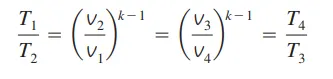
Due to constant process 1 - 2 and 3 - 4, the following formulae used

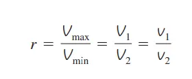
compression ratio,

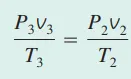
to find pressure with this relation,

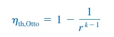
To find the efficiency of the otto cycle,

The following graph is idle otto cycle

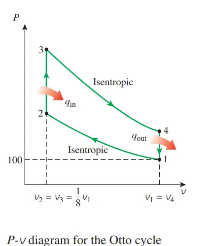
By Analysis The P-v diagram of the ideal Otto cycle,
here note that the air contained in the cylinder forms a closed system.

The maximum temperature and pressure in an Otto cycle occur at the
end of the constant-volume heat-addition process (state 3). But first, we need
to determine the temperature and pressure of air at the end of the isentropic
compression process (state 2),

Python code

import math as mt
import matplotlib.pyplot as pt

def engine_kinematics(bore,stroke,con_rod,cr,start_crank,end_crank):
	
	a = stroke/2;
	r = con_rod/a;

	v_s = (mt.pi)*(.25)*pow(bore,2)*stroke
	v_c = v_s/(cr-1)

	sc = mt.radians(start_crank)
	ec = mt.radians(end_crank)

	num_values = 100
	dtheta = (ec-sc)/(num_values-1)
	V=[]

	for i in range (0,num_values):
		theta = sc + i*dtheta
		term1 = 0.5*(cr-1)
		term2 = r + 1-mt.cos(theta)
		term3 = pow(r,2) - pow(mt.sin(theta),2)
		term3 = pow(term3,0.5)
		V.append((1 + term1*(term2-term3))*v_c)
	return(V)

# inputs
p1 = 10135
t1 = 500
t3 = 2300
gamma = 1.4

# geometric parameters
bore=.1
stroke=.1
con_rod=.15
cr=12

# volume computation
v_s = (mt.pi/4)*pow(bore,2)*stroke
v_c = v_s/(cr-1)

# state variable @ (1)
v1 = v_c+v_s

# state variable @ (2)

v2 = v_c
p2 = p1* (pow(cr,gamma))
c = p1*v1/t1
t2 = p2*v2/c
constant = p1*pow(v1,gamma)

V_compression = engine_kinematics(bore,stroke,con_rod,cr,180,0)
P_compression =[]
for V1 in V_compression:
	P_compression.append(constant/pow(V1,gamma))

# state variable @ (3)

v3=v2
p3=p2*t3/t2

# state variable @ (4)

v4=v1
p4=p3*pow(v3,gamma)/pow(v4,gamma)
constant = p3*pow(v3,gamma)

V_expansion = engine_kinematics(bore,stroke,con_rod,cr,180,360)
P_expansion = []
for V3 in V_expansion:
	P_expansion.append(constant/pow(V3,gamma))
t4=p4*v4/c
print('State points \t\t1\t\t2\t\t\t3\t\t\t4\npressure \t\t',p1,'\t',round(p2,2),'\t',round(p3,2),'\t',round(p4,2) )
print('Volume \t\t\t',round(v1,5),round(v2,5),'\t\t',round(v3,5),'\t\t',round(v4,5))
print('Temperature \t',round(t1,5),'\t',round(t2,2),'\t',round(t3,5),'\t\t',round(t4,2))
#let plot data
pt.plot(V_compression,P_compression,'g',label=r'$real-otto-cycle$')
pt.plot(V_expansion,P_expansion,'g')
pt.plot([v1,v2,v3,v4,v1],[p1,p2,p3,p4,p1],'b--',label=r'$idel-otto-cycle$')
pt.xlim(0,0.00087)
pt.ylim(0,566452)
pt.legend(loc='best')
pt.xlabel('volume')
pt.ylabel('pressure')
pt.savefig('comparision of idel vs real otto cycle.png')
pt.show()

#thermal efficieny
eta = (1-(pow(cr,(1-gamma))))*100
print('\nThermal efficiency of otto cycle',round(eta,2),'%')

Step-wise Explanation of the Code :

1. Then the given inputs or known values of gamma, t₃, p₁, t₁, are entered.
2. Then the Engine Geometric parameters are entered which include bore diameter, stroke length, connecting rod length, and the compression ratio of the engine.
3. The swept volume and clearance volume is calculated using some relations and formulas.
4. The state variables v1, v2, p2, t2, v3, p3, v4, and p4 are calculated using the formulas mentioned above.
5. Now to achieve a set of solutions for every value of the crank angle, a separate code is written in a new script.
6. Here in this script, ‘function’ syntax is used which declares a function named “engine_kinematic”
7. that accepts inputs “bore, stroke, con_rod, cr, start_thetha, end_thetha,” and returns outputs in the “V” array.
8. The value of crank angle ‘theta’ is calculated for 100 values between the initial angle and final angle.
9. Then to obtain a curve, the equation of V i.e Volume inside the cylinder when the piston is at an angle θ, is formulated.
10. This function is called in the code and V_compression, P_compression, V_expansion, P_expansion are calculated with respect to the values of crank angle ‘theta’.
11. Thermal Efficiency is calculated by using the formula mentioned above.
12. Finally, all state variable points are plotted along with the curves and the PV cycle generated for both real and ideal otto cycle.

Final results

PV plot

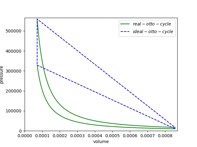
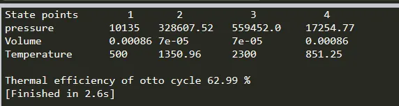
State points data and Efficiency results

CONCLUSION:

• The PV diagram for all four processes has been plotted. It is been noted that the actual PV diagram has round corners compared to the ideal P-V diagram.
• The thermal efficiency of the Otto Cycle is 62.99%. As noted, thermal efficiency mainly depends on the compression ratio of the engine and the type of fluid. So it can be concluded that engines with a higher compression ratio will have high thermal efficiency.