Air standard Cycle Characterictics using Python

Otto Cycle

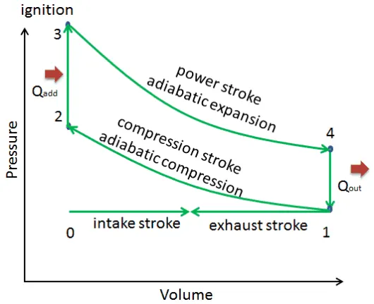
An Otto cycle is an idealized thermodynamic cycle that describes the functioning of a typical spark ignition piston engine. It is the thermodynamic cycle most commonly found in automobile engines.
The Otto cycle is a description of what happens to a mass of gas as it is subjected to changes of pressure, temperature, volume, the addition of heat, and the removal of heat. The mass of gas that is subjected to those changes is called the system. The system, in this case, is defined to be the fluid (gas) within the cylinder. By describing the changes that take place within the system, it will also describe in the inverse, the system's effect on the environment. In the case of the Otto cycle, the effect will be to produce enough net-work from the system so as to propel an automobile and its occupants in the environment.

The Otto cycle is constructed from:
Top and bottom of the loop: a pair of quasi-parallel and isentropic processes (frictionless, adiabatic reversible).
Left and right sides of the loop: a pair of parallel isochoric processes (constant volume).

Explanation of the Code

Based on the Inputs Variables we calculate the values for Swept Volume and Clearance Volume

Swept Volume=`pi/4D^2l` where

`D`= Bore Diameter

`l`=Stroke Length

Clearance Volume=`V_(cl earance)=V_(swept)/(Cr-1)`

where `Cr=` Compression Ratio

#volume compuatation
v_s=(math.pi/4)*pow(bore,2)*stroke
v_c=v_s/(cr-1)

#state point 1
v1=v_c+v_s

#state point 2
v2=v_c

Using the above we find V1 and V2. Given P1=101325, So we have a state variable of point 1.

To find the state variables at Point 2 we equate the isentropic expansion equation, that is

`P2=P1*((V1)/(V 2))^gamma`

To find the temperature at point 2 we use the Ideal Gas equation

`(P1*V1)/(T1)=(P2*V2)/(T2)=nR`

#p2v2^gama=p1v1^gama
p2=p1*pow(v1, gama)/pow(v2,gama)

#p2v2/t2=p1v1/t1 | rhs=p1v1/t1 | p2v2/t2=rhs | t2=p2v2/rhs
rhs=p1*v1/t1
t2=p2*v2/rhs

In order to get a smooth curve from point P1 to point P2, we need to find instantaneous values of Pressure and Volume corresponding to each other. To find volume at instantaneous values of the crank angle we use the below equation and create a function named "engine_kinematics".

Using the instantaneous volume we find the corresponding values of pressure.

`V=(1+0.5(Cr-1)[R+1-costheta-(R^2-sin^2theta)^0.5]`

def engine_kinematics(bore,stroke,con_rod,cr,start_crank,end_crank):
	a=stroke/2
	R=con_rod/a

	#Volume Parameters
	V_s=math.pi*(1/4)*pow(bore,2)*stroke
	V_c=V_s/(cr-1)

	sc=math.radians(start_crank)
	ec=math.radians(end_crank)

	num_values=50
	dtheta=(ec-sc)/(num_values-1)
	V=[]
	for i in range (0,num_values):
		theta=sc+i*dtheta
		term1=0.5*(cr-1)
		term2=R+1-math.cos(theta)
		term3=pow(R,2)-pow(math.sin(theta),2)
		term3=pow(term3,0.5)
		V.append((1+term1*(term2-term3))*V_c)
	return V

Similarly, we find the values State Point P3 and P4

#state point 3
v3=v2
#p3v3/t3=p2v2/t2 | rhs=p2v2/t2 | p3=rhs*t3/v3
rhs=p2*v2/t2
p3=rhs*t3/v3

V_exp=engine_kinematics(bore,stroke,con_rod,cr,0,180)
constant=p3*pow(v3,gama)
P_exp=[]
for v in V_exp:	
	P_exp.append(constant/pow(v,gama))

#state pint 4
v4=v1
#p4v4^gama=p3v3^gama
p4=p3*pow(v3,gama)/pow(v4,gama)

#p4v/t4=rhs
t4=p4*v4/rhs

Plotting

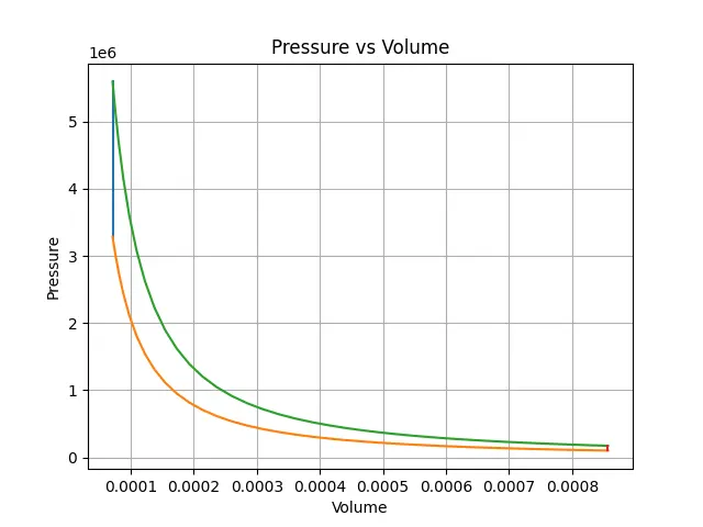
First, we plot point P1 and create the curve from point p1 to point p2 as per the instantaneous values of volume and pressure, and in the same way, we plot point P3 and P4. In the end, we join two curves.

#Plotting
plt.plot([v2,v3],[p2,p3])
plt.plot(V_comp,P_comp)
plt.plot(V_exp,P_exp)
plt.plot([v1,v4],[p1,p4])
plt.xlabel('Volume')
plt.ylabel('Pressure')
plt.title('Pressure vs Volume')
plt.grid()
plt.show()

Complete Program

#Otto Cycle
import math
import matplotlib.pyplot as plt
#inputs
p1=101325
t1=500
gama=1.4
t3=2300

#gerometric parameters
bore=0.1
stroke=0.1
con_rod=0.15
cr=12

def engine_kinematics(bore,stroke,con_rod,cr,start_crank,end_crank):
	a=stroke/2
	R=con_rod/a

	#Volume Parameters
	V_s=math.pi*(1/4)*pow(bore,2)*stroke
	V_c=V_s/(cr-1)

	sc=math.radians(start_crank)
	ec=math.radians(end_crank)

	num_values=50
	dtheta=(ec-sc)/(num_values-1)
	V=[]
	for i in range (0,num_values):
		theta=sc+i*dtheta
		term1=0.5*(cr-1)
		term2=R+1-math.cos(theta)
		term3=pow(R,2)-pow(math.sin(theta),2)
		term3=pow(term3,0.5)
		V.append((1+term1*(term2-term3))*V_c)
	return V

#volume compuatation
v_s=(math.pi/4)*pow(bore,2)*stroke
v_c=v_s/(cr-1)

#state point 1
v1=v_c+v_s

#state point 2
v2=v_c

#p2v2^gama=p1v1^gama
p2=p1*pow(v1, gama)/pow(v2,gama)

#p2v2/t2=p1v1/t1 | rhs=p1v1/t1 | p2v2/t2=rhs | t2=p2v2/rhs
rhs=p1*v1/t1
t2=p2*v2/rhs

V_comp=engine_kinematics(bore,stroke,con_rod,cr,180,0)
constant=p1*pow(v1,gama)
P_comp=[]
for v in V_comp:	
	P_comp.append(constant/pow(v,gama))


#state point 3
v3=v2
#p3v3/t3=p2v2/t2 | rhs=p2v2/t2 | p3=rhs*t3/v3
rhs=p2*v2/t2
p3=rhs*t3/v3

V_exp=engine_kinematics(bore,stroke,con_rod,cr,0,180)
constant=p3*pow(v3,gama)
P_exp=[]
for v in V_exp:	
	P_exp.append(constant/pow(v,gama))

#state pint 4
v4=v1
#p4v4^gama=p3v3^gama
p4=p3*pow(v3,gama)/pow(v4,gama)

#p4v/t4=rhs
t4=p4*v4/rhs

#Plotting
plt.plot([v2,v3],[p2,p3])
plt.plot(V_comp,P_comp)
plt.plot(V_exp,P_exp)
plt.plot([v1,v4],[p1,p4])
plt.xlabel('Volume')
plt.ylabel('Pressure')
plt.title('Pressure vs Volume')
plt.grid()
plt.show()

Result

The below graph represents a PV diagram for an air compression cycle commonly known as the otto cycle. A pressure–volume diagram is used to describe corresponding changes in volume and pressure in a system.

Thermal Efficiency of the cycle

`eta=1-T_1/T_2=1-500/1350.96=62.98%`

Modern gasoline engines have a maximum thermal efficiency of more than 50%, but road-legal cars are only about 20% to 35% when used to power a car. In other words, even when the engine is operating at its point of maximum thermal efficiency, of the total heat energy released by the gasoline consumed, about 65-80% of total power is emitted as heat without being turned into useful work, i.e. turning the crankshaft.