Week 2 Air standard Cycle

Otto Cycle:

An Otto cycle is an idealized thermodynamic cycle that describes the functioning of a typical spark ignition piston engine. This cycle mostly found in automobile engines. The Otto cycle is a description of what happens to a mass of gas as it is subjected to changes of pressure, temperature, volume, the addition of heat, and the removal of heat. The mass of gas is known as the system.

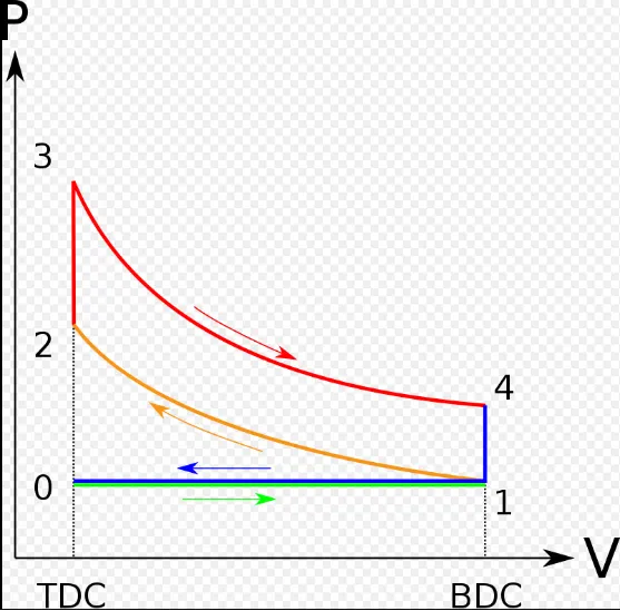
The process of the otto cycle is given below depending upon the PV diagram.

• Process 0–1 a mass of air is drawn into piston/cylinder arrangement at constant pressure.
• Process 1–2 is an adiabatic (isentropic) compression of the charge as the piston moves from the bottom dead center(BDC) to the top dead center(TDC).
• Process 2–3 is a constant-volume heat transfer to the working gas from an external source while the piston is at the top dead center. This process is intended to represent the ignition of the fuel-air mixture and the subsequent rapid burning.
• Process 3–4 is an adiabatic (isentropic) expansion (power stroke).
• Process 4–1 completes the cycle by a constant-volume process in which heat is rejected from the air while the piston is at BDC.
• Process 1–0 the mass of air is released into the atmosphere in a constant pressure process.

Efficiency (`eta`) = 1 - `Q_2/Q_1`

= 1 - `(t_4-t_1)/(t_3-t_2)`

To calculate the volume trace

`V/V_c = 1+ 1/2(r_c-1)*[R+1-costheta-(R^2-sin^2theta)^(1/2)]`

V_s(swept volume) = `pi/4`*bore^2*stroke

V_c(celerance volume) = `V_s/(cr-1)`

Code:-

# otto cycle simulator

import math  # for doing mathamatical calculations
import matplotlib.pyplot as plt  # for ploting
import numpy as np # numpy is used to +, -, *, /, power, and linspace for the arrays

def engine_kinematics(bore, stroke, con_rod, cr, start_crank, end_crank):

	# Geometric parameters
	a = stroke/2    # crarck fin radius
	R = con_rod/a   

	# volume parameters
	V_s = math.pi*(1/4)*pow(bore,2)*stroke  # swept volume 
	V_c = V_s/(cr-1)                        # cleareance volume

	sc = math.radians(start_crank)
	ec = math.radians(end_crank)

	num_values = 50
	dtheta = (ec-sc)/(num_values-1)

	V = []

	for i in range(0,num_values):
		theta = sc + i*dtheta

		term1 = 0.5*(cr-1)
		term2 = R + 1 - math.cos(theta)
		term3 = pow(pow(R,2) - pow(math.sin(theta),2),0.5)

		V.append((1 + term1*(term2 - term3))*V_c) 
	
	return V 

#inputs
p1 = 101325
t1 = 500
gamma = 1.4
t3 = 2300

#
bore = 0.1
stroke = 0.1
con_rod = 0.15 
cr = 6

# vol computation
v_s = (math.pi/4)*pow(bore,2)*stroke 
v_c = v_s/(cr-1)
v1 = v_s + v_c

# state pt 2
v2 = v_c

# p1v1^gamma = p2v2^gamma
p2 = p1*pow(v1,gamma)/pow(v2,gamma)

# p2v2/t2 = p1v1/t1
rhs = p1*v1/t1
t2 = p2*v2/rhs
V_compression = engine_kinematics(bore, stroke, con_rod, cr, 180, 0)

constant = p1*pow(v1,gamma)
#P_compression*V_compression^gamma = constant

P_compression = []
for v in V_compression:
	P_compression.append(constant/pow(v,gamma))

# state pt 3
v3 = v2

# p3v3/t3 = p2v2/t3 
rhs = p2*v2/t2
p3 = rhs*t3/v3

V_expansion = engine_kinematics(bore, stroke, con_rod, cr, 180, 0)

constant = p3*pow(v3,gamma)
#P_compression*V_compression^gamma = constant

P_expansion = []
for v in V_expansion:
	P_expansion.append(constant/pow(v,gamma))

# state pt 4
v4 = v1

# p4v4^gamma = p3v3^gamma
p4 = p3*pow(v3,gamma)/pow(v4,gamma)

# p3v3/t3 = p4v4/t4
t4 = p4*v4*rhs

# thermal efficiency
mu = 1-(1/pow(cr,(gamma-1)))
print(mu)

plt.plot([v2,v3],[p2,p3])
plt.plot(V_compression,P_compression)
plt.plot(V_expansion,P_expansion)
plt.plot([v4,v1],[p4,p1])
plt.xlabel('volume')
plt.ylabel('pressure')
plt.title('Pressure-Volume diagram')
plt.grid('on')
plt.show()

Result:-

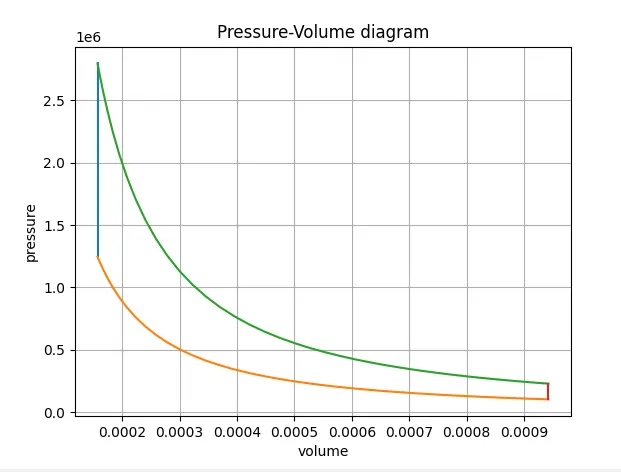
Thermal efficiency(`mu`) for compression ratio 6 = 0.511640

`mu` = 51.1640%