Week 2 Air standard Cycle
Air Standard Cycle
Gerardo Pérez Guerra
Universidad Politecnica de Queretaro
Author's Notes
Gerardo Perez Guerra, Automotive Technology Engineering, Universidad Politecnica de Queretaro.
This presentation is made by the student himself.
The Addressee of this investigation is directed to Skill Lync,
Contact: [email protected]
CONTENT
I. OBJECTIVE
The purpose of this project is being able to identify and understand the 4 state points of an Otto Cycle and write its interpretation in a programming language such as Python. This script will be able to calculate and plot :
- Pressure vs volume diagram
- The thermal efficiency of an engine
II. PROBLEM STATEMENT
The volume and pressure for each of the 4 state points must be calculated while displaying a correct form in the diagram. This also means it is necessary to evaluate the temperature at each stage to calculate its overall thermal efficiency.
III. SOLUTION PROCEDURE
III. I Introduction
An engine explained by the laws of thermodynamics is defined as a closed thermodynamic system where the quantity of matter is fixed. This implies that the work or heat can be transferred across the system where, for the case of an engine, has a flow where the matter can come in and out, these terms can also be attributed to a fluid system.[1]
For a fluid system, properties such as pressure, volume, and temperature are common and essential to determine. Therefore, for an engine, the laws of thermodynamics can describe the function of an Otto Cycle in an engine. [2]
The Otto cycle can be described as a set 4 processes by:
- Admission of the air and fuel through natural airflow
- Compression of the fuel-air mixture
- Expansion of the combusted fuel-air mixture
- The exhaust of the remaining mixture
III. II Proposed Solution
For the solution, it will be necessary to find the main variables in the system to plot in the pressure vs volume diagram. These variables are volume, pressure, and temperature.
In order to relate the volume of the cylinder with respect to the angle of the crankshaft, it is necessary to use the following equation, where V is the value to solve for:

The temperature will have an initial value of 400 kelvin, which is approximately the temperature an engine has when starting an Otto cycle. To calculate the following temperatures an equation that relates temperature with pressure will be used to solve for the temperature using initial pressure, which will be 1 atm or approx 101325 Pascals.
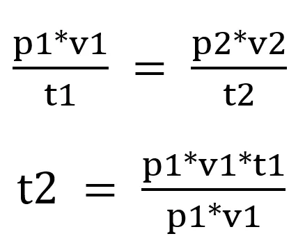
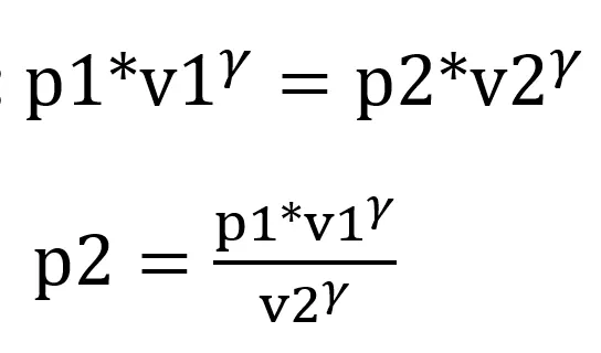
The pressure inside the engine as described will have an initial value of 1 atm or 101325 Pascals. In order to calculate the pressure (p2) in the second state point, the following formula will be used to solve for p2, where "y" the constant gamma will have a value of 1.4
In order to calculate the thermal efficiency, is necessary to use the following equation that calculates the thermal efficiency based on the output temperature and input temperature. Then it is multiplied by 100 to obtain the result in a percentage .

III. III CODING IN PYTHON
"""
Air Standard Cycle
by Gerardo Perez Guerra
"""

import math
import matplotlib.pyplot as plt

# Engine Kinematics equation
def engine_kinematics(bore, stroke, con_rod, cr, start_crank, end_crank):
	"""
       Engine kinematics equation relates the volume of an engine with the angle of the crankshaft

	"""

	# Geometric paramteters
	a = stroke/2
	R = con_rod/a

	 # Volume parameters when the crank is at starting and ending position
	V_s = math.pi*(1/4)*pow(bore,2)*stroke
	V_c = V_s/(cr-1)

	# Agnle for the crank
	sc = math.radians(start_crank)
	ec = math.radians(end_crank)

	num_values = 50

	dtheta = (ec-sc)/(num_values-1)

	V = []
	for i in range(0,num_values):
		theta = sc + i*dtheta
		term1 = 0.5*(cr-1)
		term2 = R + 1 - math.cos(theta)
		term3 = pow(pow(R,2) - pow(math.sin(theta),2),0.5)
		V.append((1 + term1*(term2 -term3))*V_c)
	return V

# Thermal efficiency equation
def thermal_efficiency(t1,t2,t3,t4):
	t_e = (1 -((t4-t1)/(t3-t2)))*100
	t_e = "%.2f" % t_e
	return t_e

# Inputs
gamma = 1.4

# Gemotric paramterers of the engine
bore = 0.1
stroke = 0.1
con_rod = 0.15
cr = 8

# Volume computation for start crank(v_s) and end crank(v_c)
v_s = (math.pi/4)*pow(bore,2)*stroke
v_c = v_s/(cr-1)

# This is the state point 1
# For volume in the engine
v1 = v_c + v_s
# Starting temeprature  in kelvin
t1 = 400
# Pressure of 1 atm in Pascals
p1 = 101325


# This is the state point 2
# Volume in the engine during compression
v2 = v_c

# Preassure is in Pascals
# p2v2^gamma = p1v1^gamma
p2 = p1*pow(v1,gamma)/pow(v2,gamma)

# Temeprature is in kelvin
# p2v2/t2 = p1v1/t1   | rhs= p1v1/t1 | p2v2/t2 =rhs | t2 = p2v2/rhs
rhs = p1*v1/t1
t2 = p2*v2/rhs

# Array of volumes from V1 to V2
V_compression = engine_kinematics(bore, stroke, con_rod, cr, 180, 0)

# Constant value
constant = p1*pow(v1,gamma)

# Array of pressures from P1 to P2
P_compression = []
for v in V_compression:
	P_compression.append(constant/pow(v,gamma))


# State point 3
v3 = v2
t3 =2300

# p3v3/t3 = p2v2/t2 | rhs = p2v2/t2 | p3 = rhs*t3/v3
rhs = p2*v2/t2
p3 = rhs*t3/v3

# Array of volumes from V3 to V4
V_expansion = engine_kinematics(bore, stroke, con_rod, cr, 0, 180)

# Constant value
constant = p3*pow(v3,gamma)

# Array of pressures from P3 to P4
P_expansion = []
for v in V_expansion:
	P_expansion.append(constant/pow(v,gamma))


# State point 4
v4 = v1

# p4v4^gamma = p3v3^gamma
p4 = p3*pow(v3,gamma)/pow(v4,gamma)

#p4v4/t4 = rhs
t4 = p4*v4/rhs


#Calculating Thermal Efficiency
T_e = "The thermal efficiency is {} %".format(thermal_efficiency(t1,t2,t3,t4))


# Graphing Pressure vs Volume Diagram
# Title at the upper side
plt.title('Pressure vs Volume Diagram')

# This defines the name of the x-axis
plt.xlabel('Volume (m^3)')

# This defines the name of the y-axis
plt.ylabel('Pressure (MPa)')

#This defines the Blue line where the preassure decreases but volume stays constant
plt.plot([v4,v1],[p4,p1], color='#00A8FF', linewidth=2, label='4 => 1 Heat absortion') # Hex colorspectrum
plt.plot([v1,v1],[p1,-p2/8],'--', color='gray', linewidth=1)
plt.plot([v1,0],[p1,p1],'--', color='gray', linewidth=1)
plt.text(v1,p1,"1")

#This defines the Orange line where the preassure increases exponencially as the volume decreases
plt.plot(V_compression, P_compression, color='orange', linewidth=3, label='1 => 2 Compression')  # String colorspectrum
plt.text(v2,p2,"2")
plt.plot([v2,0],[p2,p2],'--', color='gray', linewidth=1)

#This defines the Purple line where the preassure increases by the spark and combustion of the air-fuel mixture and volume stays constant
plt.plot([v2,v3],[p2,p3], color='#FF29FF', linewidth=3, label='2 => 3 Combustion')     # Hex colorspectrum
plt.plot([v2,v2],[p2,-p2/8], '--',color='gray', linewidth=1)
plt.plot([v3,0],[p3,p3],'--', color='gray', linewidth=1)
plt.text(v3,p3,"3")

#This defines the red line where the preassure decreases exponentially as the volume increases
plt.plot(V_expansion, P_expansion, color='#FF5600', linewidth=3, label='3 => 4 Expansion') # Hex colorspectrum
plt.text(v4,p4,"4")

#This defines the green line where the preassure stays constant as the volume increases and decreases in both directions
plt.plot([v1, v2],[p1,p1],'g', linewidth=3, label='5 <> 1 Admission and Exhaust') # Single-letter color code
plt.text(v2,p1,"5")

# Adding thermal efficiency value into the Graph
plt.text(v1,p3/2,T_e, ha='right')

# Adding signature
plt.text(v1,p2,"by Gerardo Perez Guerra", ha='right')

#This adds the labels into the graph
plt.legend()

# These are the limits of the graph.
plt.xlim(0,0.001)
plt.ylim(-p2/8,p3*1.2)

#This shows the graph
plt.show()
IV. RESULTS & DISCUSSION
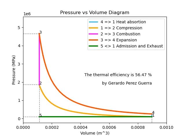
IV. I Conclusion
In conclusion, the output for the thermal efficiency is 56.47% and the Otty cycle is shown starting from point 1 where the piston receives the air-fuel mixture and compress it to point 2 where the compression is exponential. From point 2 to point 3 the mixture is combusted by a spark and transformed into mechanical energy from point 3 to point 4 so that it can come back to point 1 and intake the mixture by natural air pressure to point 5.
VI. REFERENCES
1. Quattrochi, D., 2006. 1.2 Definitions And Fundamental Ideas Of Thermodynamics. [online] Web.mit.edu. Available at: <http://web.mit.edu/16.unified/www/SPRING/propulsion/notes/node10.html> [Accessed 21 August 2020].
2. Afework, B., Amin, S. and Donev, J., 2020. Otto Cycle - Energy Education. [online] Energyeducation.ca. Available at: <https://energyeducation.ca/encyclopedia/Otto_cycle> [Accessed 22 August 2020].