Week 3 - Solving second order ODEs

Air Standard Cycle

Gerardo Pérez Guerra

Universidad Politecnica de Queretaro

Author's Notes

Gerardo Perez Guerra, Automotive Technology Engineering, Universidad Politecnica de Queretaro.

This presentation is made by the student himself.

The Addressee of this investigation is directed to Skill Lync,

Contact: [email protected]

CONTENT

I. OBJECTIVE

The purpose is to write a program in Python that will simulate the pendulum motion by solving a second-order differential equation.

The program must include the following criteria:

• L=1 meter,
• m=1 kg,
• b=0.05.
• g=9.81 m/s2.

Where "L" is the length of the pendulum, "m" is the mass of the ball, "g" is the gravitational acceleration, and "b" is the damping coefficient.

Simulate the motion between 0-20 sec, for angular displacement=0,angular velocity=3 rad/sec at time t=0.

II. PROBLEM STATEMENT

III. I Introduction

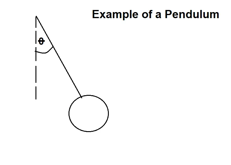
To overcome this challenge, it is crucial to solve the ODE and then use the values given to plot them so that it can be interpreted in objects moving as a pendulum.

This challenge also includes animating the figures for each value given in time by having one end fixed and the other moving according to the ODE.

III. II Proposed Solution

My proposed solution relies on understanding the values given when solving the following equation:

When solving the equation using python one must first divide the second-order equation into two different segments to solve them individually and get as a result the angle of the pendulum. These equations are then solved by the module ODE from python, an example of the equations sued are described as follow:

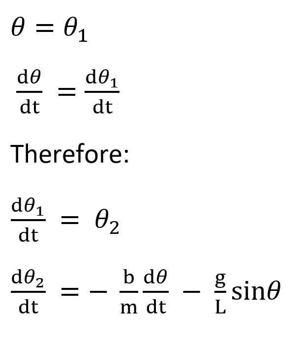
Once having these two equations, then it is possible to use the other variables established and solve for the equation using the module scipy. integrate module.

Once it is resolved, an array of numbers is going to be provided and a loop must be created with the proper coding for a graph. Then, a code must be done to loop the code to a specific set of numbers.

In order to use the array generated by the equation, the following trigonometric properties were used to coordinate and locate the position of the ball based on the angle with respect to time.

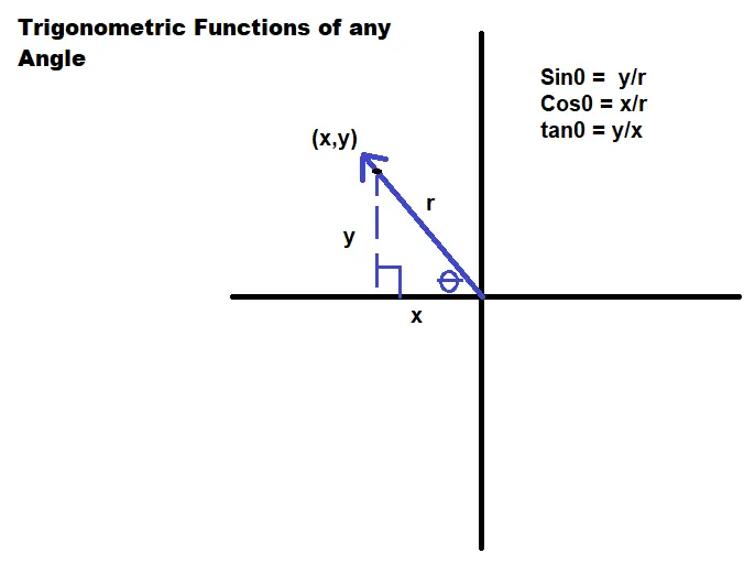
To calculate the value of x and y, it is necessary to solve for these values using trigonometric properties. it means that to calculate x, the angle and the length of the rod are needed. For the angle is the array of the first column when solving the ODE multiplied by the length of the rod (1m).

III. III CODING IN PYTHON

import matplotlib.pyplot as plt 
import math
from matplotlib.offsetbox import (TextArea, DrawingArea, OffsetImage, AnnotationBbox)
import matplotlib.image as mpimg 
import numpy as np 
from scipy.integrate import odeint


# ODE Function of Pendulum motion that returns dz/dt.
def model(theta,t,b,g,l,m):
	theta1 = theta[0]
	theta2 = theta[1]
	dtheta1_dt = theta2
	dtheta2_dt = -(b/m)*theta2 - (g/l)*math.sin(theta1)
	dtheta_dt = [dtheta1_dt, dtheta2_dt]
	return dtheta_dt

#Established variables of the pendulum.
b = 0.05
g = 9.81
l = 1
m = 1

# Time points ( 150 divisions between 0 and 10).
t = np.linspace(0,10,150)

# Initial conditions [angular displacement , angular velocity].
theta_0 = [0,3]


# Method to solve the ODE.
theta = odeint(model,theta_0,t, args = (b,g,l,m))

# This allows to put a style on the graph(background color, and grid appereance).
plt.style.use('ggplot')

# Counter variable needed for the filename.
ct = 1

#This is the loop that will give 150 images that will be converted into gif.
for j in theta[:,0]:

	# This allow us to use the angle of displacement to calculate the coordinates of the ball using trigonometric functions.
	x_1 = l*(-math.sin(j))
	y_1 = l*(-math.cos(j))

	# This represents the coordiantes of the fixed end of the pendulum.
	x_0 = 0
	y_0 = 1.75

	fig, ax = plt.subplots()

	# These are the limits of the graph.
	ax.set_xlim(-2, 3)
	ax.set_ylim(-2, 3.5)	

	# This generates the filename for each graph using the counter variable. 
	filename = "test%05d.png" % ct
	ct = ct + 1

	# Title at the upper side
	plt.title('Simulation of Pendulum Motion')

	# This calls for an image (jpg format) and names it with the variable "wall".
	wall = mpimg.imread('wall.jpg')

	# This gives the image a size.
	imagebox = OffsetImage(wall, zoom = 0.22)

	# This places the image into a specific coordinate.
	location_wall = AnnotationBbox(imagebox, (0,2.5))

	# This adds the image into the graph.
	ax.add_artist(location_wall)	

	#This defines the characteristics of the rod
	plt.plot([x_0,x_1],[y_0,y_1],'b-',linewidth=10, label = 'Rod')

	#This defines the characteristics of the ball
	plt.plot( x_1, y_1, marker = 'o', markerfacecolor = 'red', markersize = '25', label = 'Ball')

	#This defines the characteristics of the second ball only for aesthetics
	plt.plot( x_1, y_1,'o', markerfacecolor = 'tomato',markersize = '10')

	#This defines the characteristics of the center line as reference for the pendulum
	plt.plot([x_0,x_0],[y_0,-2],'--', color='black', linewidth=1)
	
	# Adding signature
	plt.text(2,-1,"by Gerardo Perez Guerra", ha='right')

	#This adds the labels into the graph while stating the characteristics of the description box
	plt.legend(loc=4, fontsize= 'large', ncol=2, fancybox= True, shadow = True, framealpha = 0.75)

	# This saves the graph with the filename format
	plt.savefig(filename)

# To convert the images into an animation using either code in CMD
# convert * pendulum.gif
# magick *.png pendulum.gif

IV. RESULTS & DISCUSSION

IV. I Errors

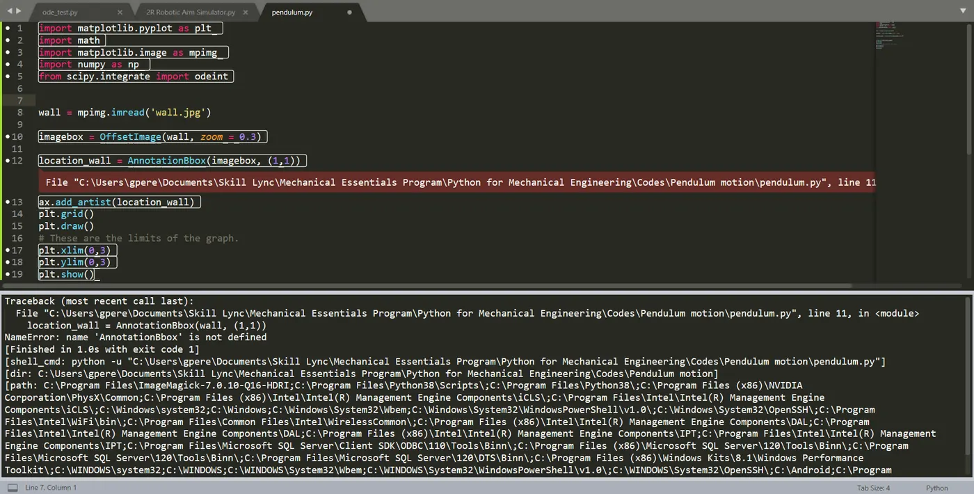
One of the first errors I encountered was the "NameError" type for a specific function. This was quickly solved after reading the error code and realizing that I needed to import the correct module.

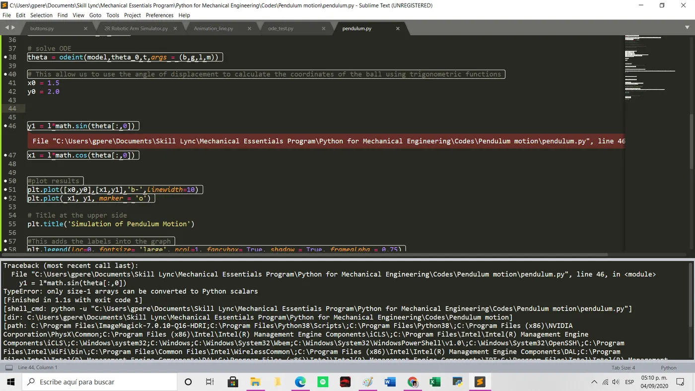
For this error, I realized that I was using a size-2 array ( angular displacement, and angular velocity) for a size-1 function. The array "Theta" has the arrays of angular displacement and angular velocity within it. This was solved when using the " For loop" method, assigning the the array for angular displacement to the variable "j" , and finally using the j value in the trigonometric function to find x and y.

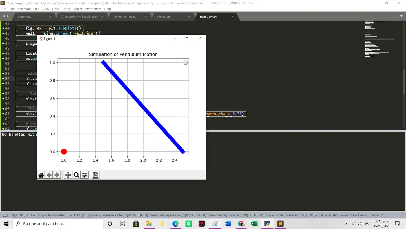
Finally one of the biggest problems I faced and which I wasn`t expecting completely was the actual representation of the movement of the pendulum. I was realizing that even when plotting the values into the graph I was displaying the movement in the wrong direction. To solve this I had to assign the sine function to the x variable and the cosine fucntion to the y variable. This placed the movement vertically but upside down. In order to change this I placed a "-" sign to the function in order to switch the movement up. The result was the correct perception of movement of a pendulum.

IV. II Video link

https://youtu.be/wiAR9drpih0

IV. III Conclusion

This challenge allowed me to understand many things, one of them is the orientation of the movement. One must account that the motion might not always be in the same orientation as expected in real life. The process of which any high-order ODE can be divided into several and smaller fractions of simple ODES is an excellent way to solve them. I believe that troubleshooting and understanding the error types in python is key.

VI. REFERENCES

N/A