Validation studies of Symmetry BC vs Wedge BC in OpenFOAM vs Analytical H.P equation
Simulation of Laminar Flow through a Pipe in OpenFoam
Liquid or gas flow through pipes or ducts is commonly used in heating and cooling applications and fluid distribution networks. The fluid in such applications is usually forced to flow by a fan or pump through a flow section. The friction, which is directly related to the pressure drop and head loss during flow through pipes and ducts. The pressure drop is then used to determine the pumping power requirement. A typical piping system involves pipes of different diameters connected to each other by various fittings or elbows to route the fluid, valves to control the flow rate, and pumps to pressurize the fluid.
The fluid velocity in a pipe changes from zero at the wall because of the no-slip condition to a maximum at the pipe center. In fluid flow, it is convenient to work with an average velocity `V_(avg)`, which remains constant in incompressible flow when the cross-sectional area of the pipe is constant.
Laminar Flow
Laminar or streamline flow in pipes (or tubes) occurs when a fluid flows in parallel layers, with no disruption between the layers. At low velocities, the fluid tends to flow without lateral mixing, and adjacent layers slide past one another. There are no cross-currents perpendicular to the direction of flow, nor eddies or swirls of fluids. In laminar flow, the motion of the particles of the fluid is very orderly with all particles moving in straight lines parallel to the pipe walls. Any lateral mixing (mixing at right angles to the flow direction) occurs by the action of diffusion between layers of the liquid. Diffusion mixing can be slow however if the diameter of the pipe of the tube is small then this diffusive mixing can be very significant.
Turbulent Flow
Turbulent flow is a flow regime characterized by chaotic property changes. This includes a rapid variation of pressure and flows velocity in space and time. Turbulent flow is a type of fluid (gas or liquid) flow in which the fluid undergoes irregular fluctuations, or mixing, in contrast to laminar flow, in which the fluid moves in smooth paths or layers. In turbulent flow, the speed of the fluid at a point is continuously undergoing changes in both magnitude and direction.
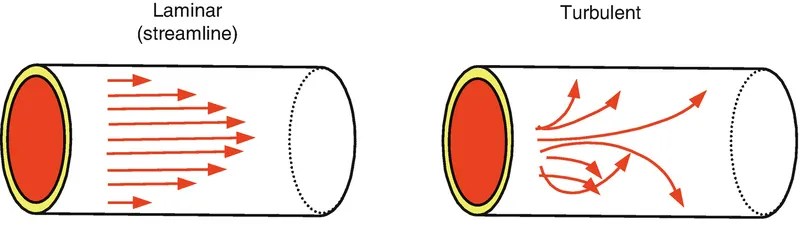
Most kinds of fluid flow are turbulent, except for laminar flow at the leading edge of solids moving relative to fluids or extremely close to solid surfaces, such as the inside wall of a pipe, or in cases of fluids of high viscosity (relatively great sluggishness) flowing slowly through small channels. Common examples of turbulent flow are blood flow in arteries, oil transport in pipelines, lava flow, atmosphere and ocean currents, the flow through pumps and turbines, and the flow in boat wakes and around aircraft-wing tips.
Reynolds Number
The Reynolds number is the ratio of inertial forces to viscous forces within a fluid that is subjected to relative internal movement due to different fluid velocities. A region where these forces change behaviour is known as a boundary layer, such as the bounding surface in the interior of a pipe.
The Reynolds number (`Re`) helps predict flow patterns in different fluid flow situations. At low Reynolds numbers, flows tend to be dominated by laminar (sheet-like) flow, while at high Reynolds numbers flows tend to be turbulent.
`Re=(rhoV_(avg)^2L^2)/(muV_(avg)L)=(rhoV_(avg)L)/(mu)=(V_(avg)L)/(nu)`
Reynolds Number for a internal flow through circular pipe is given as, `Re=(rhoV_(avg)D)/(mu)`
Reynolds number for flow through pipes
`Re<=2300` Laminar flow
`2300<=Re<=4000` Transitional flow
`Re>=4000` Turbulent Flow
Entrance Length
The entrance length is the distance a flow travels after entering a pipe before the flow becomes fully developed. Entrance length refers to the length of the entry region, the area following the pipe entrance where effects originating from the interior wall of the pipe propagate into the flow as an expanding boundary layer. When the boundary layer expands to fill the entire pipe, the developing flow becomes a fully developed flow, where flow characteristics no longer change with increased distance along the pipe. Many different entrance lengths exist to describe a variety of flow conditions.
The region from the pipe inlet to the point at which the velocity profile is fully developed is called the hydrodynamic entrance region, and the length of this region is called the hydrodynamic entry length `L_h`.
Velocity profile for Laminar flow
The hydrodynamic entry length is usually taken to be the distance from the pipe entrance to where the wall shear stress (and thus the friction factor) reaches within about 2% of the fully developed value.
For Laminar Flow
`L_(h,laminar)/D=0.05Re`
For `Re` 20, the hydrodynamic entry length is about the size of the diameter but increases linearly with velocity. In the limiting laminar case of `Re` 2300, the hydrodynamic entry length is 115D.
For Turbulent Flow
In turbulent flow, the intense mixing during random fluctuations usually overshadows the effects of molecular diffusion. The nondimensional hydrodynamic entry length for turbulent flow is approximated as
`L_(h,turbu l ent)/D=1.359Re^(1/4)`
The entrance effects become insignificant beyond a pipe length of about 10 diameters, and the nondimensional hydrodynamic entry length is approximated as
`L_(h,turbu l ent)/D=10`
Velocity Profile for Laminar Flow through Pipe
The velocity profile in a fully developed laminar flow in a pipe is parabolic with a maximum at the centerline and a minimum (zero) at the pipe wall. Also, the axial velocity `u` is positive for any `r`, and thus the axial pressure gradient `(dP)/dx` must be negative that is the pressure must decrease in the flow direction because of viscous effects—it takes pressure to push the fluid through the pipe.
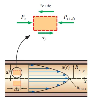
Velocity Profile
`u(r)=-R^2/(4mu)(dp)/dx(1-(r^2)/(R^2))`
`u(r)=2V_(avg)(1-r^2/R^2)`
The velocity profile since `V_(avg)` can be determined easily from the flow rate information. The maximum velocity occurs at the centerline and is determined by substituting `r=0`.
`u_max=2V_(avg)`
The average velocity in fully developed laminar pipe flow is one-half of the maximum velocity.
The fluid velocity in a pipe changes from zero at the wall because of the no-slip condition to a maximum at the pipe centre. In fluid flow, it is convenient to work with an average velocity Vavg, which remains constant in incompressible flow when the cross-sectional area of the pipe is constant.
Pressure Drop
A quantity of interest in the analysis of pipe flow is the pressure drop `DeltaP` since it is directly related to the power requirements of the fan or pump to maintain flow.
`DeltaP=P_2-P_1`
`(dP)/(dx)=(P_2-P_1)/L`
A pressure drop due to viscous effects represents an irreversible pressure loss.
Head Loss
The head loss `h_L` represents the additional height that the fluid needs to be raised by a pump in order to overcome the frictional losses in the pipe.
`h_L=(DeltaP_L)/(rhog)`
Hagen- Poiseuille's Equation
`DeltaP=(8muLQ)/(piR^4)` where
`DeltaP=` pressure difference between the two ends
`L=` length of pipe
`mu=` dynamic viscosity
`Q=` volumetric flow rate
`pi=` pi
`R=` pipe radius
Hagen Poiseuille states that for a specified flow rate, the pressure drops and thus the required pumping power is proportional to the length of the pipe and the viscosity of the fluid, but it is inversely proportional to the fourth power of the radius (or diameter) of the pipe. Therefore, the pumping power requirement for a laminar-flow piping system can be reduced by a factor of 16 by doubling the pipe diameter.
Results
Hydrodynamic Length
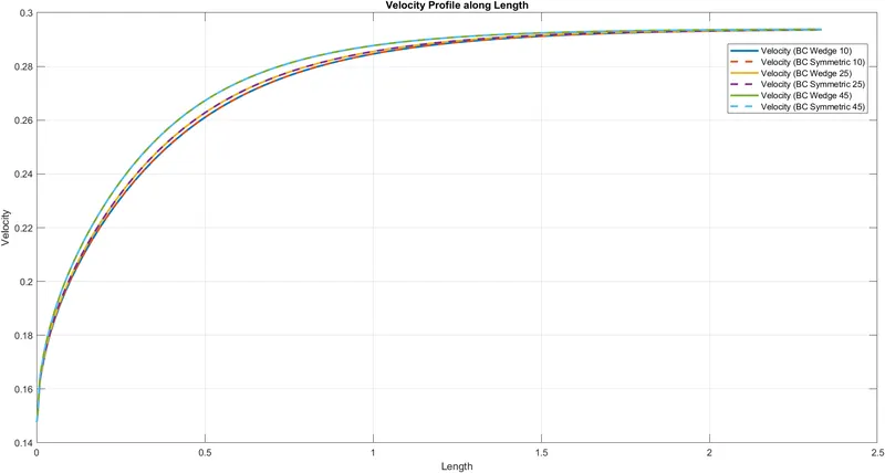
Analytical Hydrodynamic Length is found to be 1.3335m and the numerical velocity profile shows a similar result as the velocity almost becomes constant. All the cases show a similar trend irrespective of the angle and boundary condition.
%Given Inputs
re=2100;    %Reynolds Number

%Assumptions
d=0.0254/2;   %Diamter of the Pipe
r=d/2;      %Radius of the Pipe
% Dynamic viscosity
mu = 0.89e-3;
% Density
rho = 997;

% Hagen poiseuille flow equations
v_avg = (re*mu)/(rho*d);
v_max = 2*(v_avg);

%Entry Length for Laminar Flow
l_entry=0.05*re*d  %x-direction or flow direction
l=l_entry+1; %Assuming 0.25 extra for fully developed flow profile

l_entry =

    1.3335
Numerical velocity profile along the length of pipe showing that velocity becomes constant for fully developed flow corresponding to the hydrodynamic length. It is observed that the boundary condition 'wedge' and 'symmetric. offers the same results as the two lines are exactly identical.
Fully Developed Radial Velocity Profile and Max Velocity
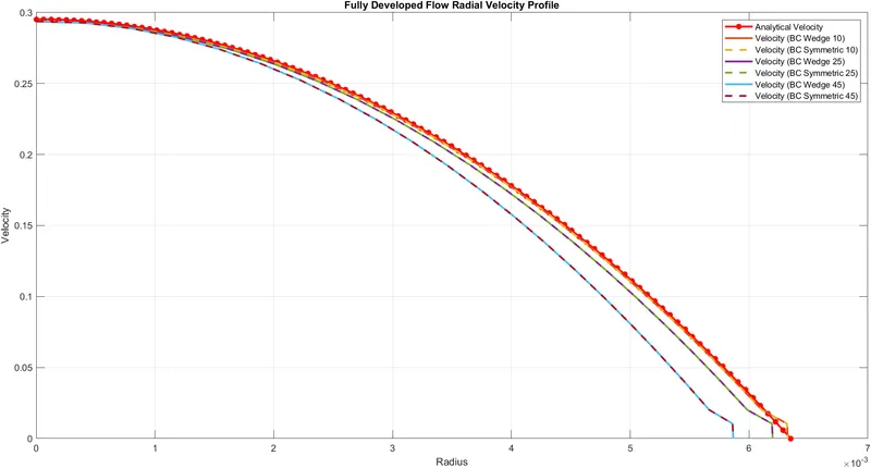
The below graph shows the radial velocity profile for a fully developed flow. It is observed that when the wedge angle is smaller the numerical results are more accurate compared to larger wedge angles.
It is observed that the boundary condition 'wedge' and 'symmetric. offers the same results as the two lines are exactly identical.
The maximum analytical flow velocity is found to be 0.2952 m/s and approximately the numerical results also show the same value.
%Given Inputs
re=2100;    %Reynolds Number

%Assumptions
d=0.0254/2;   %Diamter of the Pipe
r=d/2;      %Radius of the Pipe
% Dynamic viscosity
mu = 0.89e-3;
% Density
rho = 997;

% Hagen poiseuille flow equations
v_avg = (re*mu)/(rho*d);
v_max = 2*(v_avg)

v_max =

    0.2952

%Analytically Calculating Velocity Profile
R = linspace(0,(d/2),101);

for i = 1:length(R)
    u(i)=2*v_avg*(1-(R(i)^2/r^2));
end

%Radial Velocity Profile
figure(3)
plot(R,u,'r*-','LineWidth',2)
hold on
rad_vel_10=readmatrix('10_radial_velocity.csv');
rad_vel_10b=readmatrix('10b_radial_velocity.csv');
rad_vel_25=readmatrix('25_radial_velocity.csv');
rad_vel_25b=readmatrix('25b_radial_velocity.csv');
rad_vel_45=readmatrix('45_radial_velocity.csv');
rad_vel_45b=readmatrix('45b_radial_velocity.csv');
plot(rad_vel_10(:,1),rad_vel_10(:,2),'LineWidth',2)
plot(rad_vel_10b(:,1),rad_vel_10b(:,2),'--','LineWidth',2)
plot(rad_vel_25(:,1),rad_vel_25(:,2),'LineWidth',2)
plot(rad_vel_25b(:,1),rad_vel_25b(:,2),'--','LineWidth',2)
plot(rad_vel_45(:,1),rad_vel_45(:,2),'LineWidth',2)
plot(rad_vel_45b(:,1),rad_vel_45b(:,2),'--','LineWidth',2)
legend ('Analytical Velocity','Velocity (BC Wedge 10)','Velocity (BC Symmetric 10)','Velocity (BC Wedge 25)','Velocity (BC Symmetric 25)','Velocity (BC Wedge 45)','Velocity (BC Symmetric 45)')
xlabel('Radius')
ylabel('Velocity')
title('Fully Developed Flow Radial Velocity Profile')
grid on
Pressure Drop
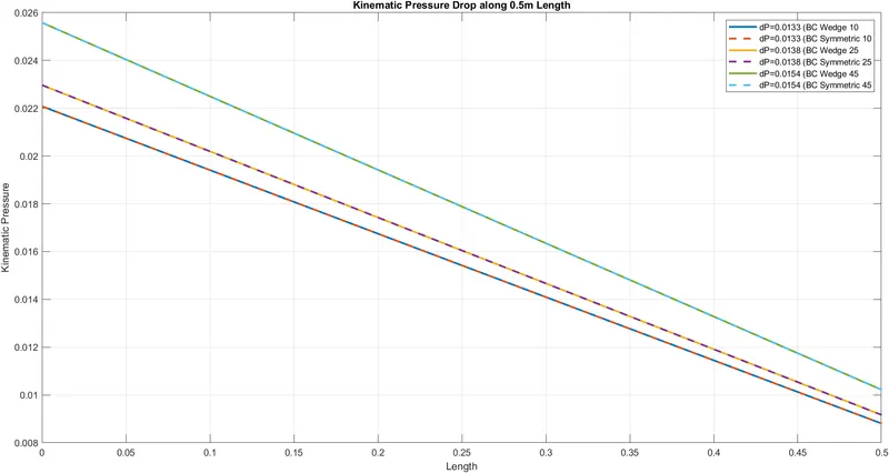
The below graph shows the pressure drop for a fully developed flow across a length of 0.5 meters. It is observed that when the wedge angle is smaller the numerical results are more accurate compared to larger wedge angles.
The analytical pressure drop for a fully developed flow is found to be 0.0131 `m^2/s^2` and approximately the numerical results also show the same value.
%Given Inputs
re=2100;    %Reynolds Number

%Assumptions
d=0.0254/2;   %Diamter of the Pipe
r=d/2;      %Radius of the Pipe
% Dynamic viscosity
mu = 0.89e-3;
% Density
rho = 997;

% Hagen poiseuille flow equations
v_avg = (re*mu)/(rho*d);
v_max = 2*(v_avg)

%Pressure Drop in Fully Developed Flow
del_p = (8*mu*0.5*v_avg)/(r^2);     %Pressure Drop
kinematic_p = del_p/rho             %Kinematic Pressure Drop

kinematic_p =

    0.0131

figure(4)
pressure_x_10=readmatrix('10_pressure_x.csv');
pressure_x_10b=readmatrix('10b_pressure_x.csv');
pressure_x_25=readmatrix('25_pressure_x.csv');
pressure_x_25b=readmatrix('25b_pressure_x.csv');
pressure_x_45=readmatrix('45_pressure_x.csv');
pressure_x_45b=readmatrix('45b_pressure_x.csv');
plot(pressure_x_10(:,1),pressure_x_10(:,2),'LineWidth',2)
hold on
plot(pressure_x_10b(:,1),pressure_x_10b(:,2),'--','LineWidth',2)
plot(pressure_x_25(:,1),pressure_x_25(:,2),'LineWidth',2)
plot(pressure_x_25b(:,1),pressure_x_25b(:,2),'--','LineWidth',2)
plot(pressure_x_45(:,1),pressure_x_45(:,2),'LineWidth',2)
plot(pressure_x_45b(:,1),pressure_x_45b(:,2),'--','LineWidth',2)
grid on
Shear Stress
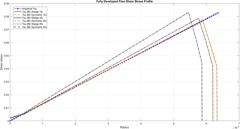
The below graph shows the shear stress profile for a fully developed flow. It is observed that when the wedge angle is smaller the numerical results are more accurate compared to larger wedge angles.
It is observed that the boundary condition 'wedge' and 'symmetric. offers the same results as the two lines are exactly identical.
The maximum analytical flow velocity is found near the wall to be 0.0828 Pa and approximately the numerical results also show the same value.
%Given Inputs
re=2100;    %Reynolds Number

%Assumptions
d=0.0254/2;   %Diamter of the Pipe
r=d/2;      %Radius of the Pipe
% Dynamic viscosity
mu = 0.89e-3;
% Density
rho = 997;

% Hagen poiseuille flow equations
v_avg = (re*mu)/(rho*d);
v_max = 2*(v_avg)

%Analytically Calculating Shear Stress and Velocity Profile
R = linspace(0,(d/2),101);

for i = 1:length(R)
    tau(i) = 2*mu*v_max*(abs(R(i)))/r^2;
end

Max_Shear=max(tau)

Max_Shear =

    0.0828

%Shear Stress Profile
figure(2)
plot(R,tau,'b*-','LineWidth',1)
hold on
tau_10=readmatrix('10_Tau.csv');
tau_10b=readmatrix('10b_Tau.csv');
tau_25=readmatrix('25_Tau.csv');
tau_25b=readmatrix('25b_Tau.csv');
tau_45=readmatrix('45_Tau.csv');
tau_45b=readmatrix('45b_Tau.csv');
plot(tau_10(:,1),tau_10(:,2),'LineWidth',2)
plot(tau_10b(:,1),tau_10b(:,2),'--','LineWidth',2)
plot(tau_25(:,1),tau_25(:,2),'LineWidth',2)
plot(tau_25b(:,1),tau_25b(:,2),'--','LineWidth',2)
plot(tau_45(:,1),tau_45(:,2),'LineWidth',2)
plot(tau_45b(:,1),tau_45b(:,2),'--','LineWidth',2)
xlabel('Radius')
ylabel('Shear stress')
grid on
legend ('Analytical Tau','Tau (BC Wedge 10)','Tau (BC Symmetric 10)','Tau (BC Wedge 25)','Tau (BC Symmetric 25)','Tau (BC Wedge 45)','Tau (BC Symmetric 45)')
title('Fully Developed Flow Shear Stress Profile')
The difference between a wedge and symmetric boundary condition
The wedge and symmetric boundary condition both are used to define an axisymmetric situation. The model and flow must be axisymmetric along a central line such that all physical variables of the flow have the same value and distribution. The difference is that in a wedge, we need to define the coordinates with respect to the angle.
A wedge is mostly for 2 dimensional axi-symmetric cases where as symmetric for any (non-planar) patch which uses the symmetry plane (slip) condition.