Week 11 - Simulation of Flow through a pipe in OpenFoam
Introduction :-
Fluid flow analysis is an important part of scientific world since it is a process used to simulate behaviours of various equipment and systems. Thus, flow is generally divided into two different types: laminar and turbulent flows.
Laminar flow is the type of fluid flow in which the fluid travels smoothly or is characterized by smooth streamlines and highly ordered motion and turbulent flow is the type of flow in which the fluid undergoes irregular fluctuations and mixing. The aim of this project is to simulate the laminar viscous flow through a regular pipe using symmetry and wedge boundary conditions and then compare the results with the analytical one obtained using Hagen-Poiseuille formula. The simulations are run in OpenFOAM and post-processed in Paraview and MATLAB is used to automate the mesh generation.
OBJECTIVES :-
The objectives of this project are as follows:
- Automate mesh generation process using MATLAB
- Perform Wedge versus Symmetry boundary conditions study
- Understand fully-developed flow and Hydro-dynamic entrance length
- Compare the results with the analytical result from Hagen-Poiseuille formula
THEORY :-
This project in simple words is about the simulation of flow through a constant cross-section pipe. The corresponding solver to such problem in OpenFOAM is icoFOAM. Hence it chosen & wedge is created according to the given wedge angle condition (less than 5°).
Dimensions of the considered Pipe :-
We assumed the diameter to be D = 10 mm.
As for the length of the pipe, we have used the entry formula as shown below:
The inlet Reynold’s number is taken as 2100.
Hence
By approximation the length of the pipe is taken as L = 1.5m.
Calculation of inlet velocity :-

Hence

Consideration imposed on wadge angle value, the wedge angle for the entire study is chosen as 2°.
Mesh Specifications :-
- The number of cells along the x direction (longer dimension) = 50
- The number cells along the y direction = 400
Generation of blockMeshDict file using MATLAB :-
In this process, the file parsing technique is used to generate the required file. This file contains the mesh specifications & the program is written in MATALAB in such a way that for each value of the wedge angle the vertices coordinates are generated automatically.
MATLAB Program :-
close all;
clear all;
clc;
theta=2;
L=1500;
dia=10;
r=dia/2;
y=r*cosd(theta/2);
z=r*sind(theta/2);


f1=fopen('blockmeshdict.txt','wt');

fprintf(f1,'/*--------------------------------*- C++ -*----------------------------------*n');
 fprintf (f1,'=========                |n')
 fprintf (f1,'      /  F ield         | OpenFOAM: The Open Source CFD Toolboxn');
  fprintf (f1,'    /   O peration     | Website:  https://openfoam.orgn');
  fprintf  (f1,'   /    A nd           | Version:  7n');
   fprintf  (f1,'  /     M anipulation  |n');
fprintf(f1, '')
fprintf(f1,'*---------------------------------------------------------------------------*n');
fprintf(f1,'FoamFilen{n')
   fprintf(f1,' version     2.0;n');
   fprintf(f1,' format      ascii;n');
    fprintf(f1,' class       dictionary;n');
    fprintf(f1,' object      blockMeshDict;n}n');

fprintf(f1,'// * * * * * * * * * * * * * * * * * * * * * * * * * * * * * * * * * * * * * //n');
fprintf(f1,'convertToMeters 0.001;nn');
fprintf(f1,'verticesn');
fprintf(f1,'(n');
fprintf(f1,'    (0 0 0)n')
fprintf(f1,'    (0 %g -%g)n',y,z)
fprintf(f1,'    (0 %g %g)n',y,z)
fprintf(f1,'    (%g 0 0)n',L)
fprintf(f1,'    (%g %g -%g)n',L,y,z)
fprintf(f1,'    (%g %g %g)n',L,y,z)
fprintf(f1,');n');
fprintf(f1,'blocksn');
fprintf(f1,'(n');
fprintf(f1,'    hex (0 1 2 0 3 4 5 3) (50 1 400) simpleGrading (0.1 1 10)n')
fprintf(f1,');n');
fprintf(f1,'edgesn');
fprintf(f1,'(n');
fprintf(f1,'    arc 1 2 (0 %g 0)n',r)
fprintf(f1,'    arc 4 5 (%g %g 0)n',L,r)
fprintf(f1,');n');
fprintf(f1,'boundaryn');
fprintf(f1,'(n');
fprintf(f1,'inletn   {n');
        fprintf(f1,'     type patch;n');
        fprintf(f1,'     facesn(n');
            fprintf(f1,'      (0 2 1 0)n);n   }n');


   fprintf(f1,'outletn{n');
        fprintf(f1,'     type patch;n');
        fprintf(f1,'     facesn   (n');
             fprintf(f1,'     (3 4 5 3)n);n}n');
   fprintf(f1,'upperWalln{n');
      fprintf(f1,'       type wall;n');
       fprintf(f1,'      facesn   (n');
            fprintf(f1,'      (1 2 5 4)n);n}n');
     fprintf(f1,'lowerWalln{n');
      fprintf(f1,'       type empty;n');
       fprintf(f1,'      facesn(n');
            fprintf(f1,'      (0 3 3 0)n);n}nn');
fprintf(f1,'frontn{n');
      fprintf(f1,'       type wedge;n');
       fprintf(f1,'      facesn(n');
            fprintf(f1,'      (0 3 5 2)n);n}nn');
            fprintf(f1,'   Backn{n');
      fprintf(f1,'       type wedge;n');
       fprintf(f1,'      facesn(n');
            fprintf(f1,'       (0 1 4 3)n);n}n);n');

fprintf(f1,'mergePatchPairsn(n);n');


fprintf(f1,'// ************************************************************************* //');
The blockMeshDict file obtained after running the above program is chown below:
/*--------------------------------*- C++ -*----------------------------------*
===============                |
            /  F ield        | OpenFOAM: The Open Source CFD Toolbox
         /   O peration     | Website:  https://openfoam.org
      /    A nd            | Version:  7
   /     M anipulation    |
*---------------------------------------------------------------------------*
FoamFile
{
 version     2.0;
 format      ascii;
 class       dictionary;
 object      blockMeshDict;
}
// * * * * * * * * * * * * * * * * * * * * * * * * * * * * * * * * * * * * * //
convertToMeters 0.001;

vertices
(
    (0 0 0)
    (0 4.99924 -0.087262)
    (0 4.99924 0.087262)
    (1500 0 0)
    (1500 4.99924 -0.087262)
    (1500 4.99924 0.087262)
);
blocks
(
    hex (0 1 2 0 3 4 5 3) (50 1 400) simpleGrading (1 1 1)
);
edges
(
    arc 1 2 (0 5 0)
    arc 4 5 (1500 5 0)
);
boundary
(
inlet
   {
     type patch;
     faces
(
      (0 2 1 0)
);
   }
outlet
{
     type patch;
     faces
   (
     (3 4 5 3)
);
}
upperWall
{
       type wall;
      faces
   (
      (1 2 5 4)
);
}
lowerWall
{
       type empty;
      faces
(
      (0 3 3 0)
);
}

front
{
       type wedge;
      faces
(
      (0 3 5 2)
);
}

   Back
{
       type wedge;
      faces
(
       (0 1 4 3)
);
}
);
mergePatchPairs
(
);
// ************************************************************************* //
ControlDict File
This file contains the time step and the time of simulation and let us modify these parameters according to what we want. In our case, the starting time is 0, the end time is 9s which means that the simulation is run for 9 seconds. The time step is taken as 0.001
/*--------------------------------*- C++ -*----------------------------------*
  =========                 |
  \      /  F ield         | OpenFOAM: The Open Source CFD Toolbox
   \    /   O peration     | Website:  https://openfoam.org
    \  /    A nd           | Version:  9
     \/     M anipulation  |
*---------------------------------------------------------------------------*/
FoamFile
{
    format      ascii;
    class       dictionary;
    location    "system";
    object      controlDict;
}
// * * * * * * * * * * * * * * * * * * * * * * * * * * * * * * * * * * * * * //

application     icoFoam;

startFrom       startTime;

startTime       0;

stopAt          endTime;

endTime         9;

deltaT          0.001;

writeControl    timeStep;

writeInterval   200;

purgeWrite      0;

writeFormat     ascii;

writePrecision  6;

writeCompression off;

timeFormat      general;

timePrecision   6;

runTimeModifiable true;


// ************************************************************************* //
Transport Properties File:
/*--------------------------------*- C++ -*----------------------------------*
  =========                 |
  \      /  F ield         | OpenFOAM: The Open Source CFD Toolbox
   \    /   O peration     | Website:  https://openfoam.org
    \  /    A nd           | Version:  9
     \/     M anipulation  |
*---------------------------------------------------------------------------*/
FoamFile
{
    format      ascii;
    class       dictionary;
    location    "constant";
    object      transportProperties;
}
// * * * * * * * * * * * * * * * * * * * * * * * * * * * * * * * * * * * * * //

nu              [0 2 -1 0 0 0 0] 8.9e-7;


// ************************************************************************* //
fvSchemes File
/*--------------------------------*- C++ -*----------------------------------*
  =========                 |
  \      /  F ield         | OpenFOAM: The Open Source CFD Toolbox
   \    /   O peration     | Website:  https://openfoam.org
    \  /    A nd           | Version:  9
     \/     M anipulation  |
*---------------------------------------------------------------------------*/
FoamFile
{
    format      ascii;
    class       dictionary;
    location    "system";
    object      fvSchemes;
}
// * * * * * * * * * * * * * * * * * * * * * * * * * * * * * * * * * * * * * //

ddtSchemes
{
    default         Euler;
}

gradSchemes
{
    default         Gauss linear;
    grad(p)         Gauss linear;
}

divSchemes
{
    default         none;
    div(phi,U)      Gauss linear;
}

laplacianSchemes
{
    default         Gauss linear orthogonal;
}

interpolationSchemes
{
    default         linear;
}

snGradSchemes
{
    default         orthogonal;
}


// ************************************************************************* //
fvSolution
/*--------------------------------*- C++ -*----------------------------------*
  =========                 |
  \      /  F ield         | OpenFOAM: The Open Source CFD Toolbox
   \    /   O peration     | Website:  https://openfoam.org
    \  /    A nd           | Version:  9
     \/     M anipulation  |
*---------------------------------------------------------------------------*/
FoamFile
{
    format      ascii;
    class       dictionary;
    location    "system";
    object      fvSolution;
}
// * * * * * * * * * * * * * * * * * * * * * * * * * * * * * * * * * * * * * //

solvers
{
    p
    {
        solver          PCG;
        preconditioner  DIC;
        tolerance       1e-06;
        relTol          0.05;
    }

    pFinal
    {
        $p;
        relTol          0;
    }

    U
    {
        solver          smoothSolver;
        smoother        symGaussSeidel;
        tolerance       1e-05;
        relTol          0;
    }
}

PISO
{
    nCorrectors     2;
    nNonOrthogonalCorrectors 0;
    pRefCell        0;
    pRefValue       0;
}


// ************************************************************************* //
Initial & Boundary conditions :-
These two types of conditions are found in p and U files which are located in 0 folder. The initial conditions are identified under Internal Field and the boundary conditions are identified under Boundary Field.
As shown by the files below, the pressure at the starting point is set to 0 and for boundary conditions, the wedge boundary condition is used on the front and back wedges of our geometry. No-slip boundary condition is used at the top wall and empty BC at the bottom walls.
The inlet velocity is set as 0.1869m/s and pressure is extrapolated from the inner nodes as well as the outlet velocity.
pfile
/*--------------------------------*- C++ -*----------------------------------*
  =========                 |
  \      /  F ield         | OpenFOAM: The Open Source CFD Toolbox
   \    /   O peration     | Website:  https://openfoam.org
    \  /    A nd           | Version:  9
     \/     M anipulation  |
*---------------------------------------------------------------------------*/
FoamFile
{
    format      ascii;
    class       volScalarField;
    object      p;
}
// * * * * * * * * * * * * * * * * * * * * * * * * * * * * * * * * * * * * * //

dimensions      [0 2 -2 0 0 0 0];

internalField   uniform 0;

boundaryField
{
    inlet
    {
        type            zeroGradient;
    }

    outlet
    {
        type            fixedValue;
        value           uniform 0;
    }

    upperWall
    {
        type            zeroGradient;
    }
    lowerWall
    {
        type            empty;
    }
    front
    {
        type            wedge;
    }
     Back
    {
        type            wedge;
    }
}

// ************************************************************************* //
Ufile
/*--------------------------------*- C++ -*----------------------------------*
  =========                 |
  \      /  F ield         | OpenFOAM: The Open Source CFD Toolbox
   \    /   O peration     | Website:  https://openfoam.org
    \  /    A nd           | Version:  9
     \/     M anipulation  |
*---------------------------------------------------------------------------*/
FoamFile
{
    format      ascii;
    class       volVectorField;
    object      U;
}
// * * * * * * * * * * * * * * * * * * * * * * * * * * * * * * * * * * * * * //

dimensions      [0 1 -1 0 0 0 0];

internalField   uniform (0 0 0);

boundaryField
{
    inlet
    {
        type            fixedValue;
        value           uniform (0.186 0 0);
    }

    outlet
    {
        type            zeroGradient;
    }

    upperWall
    {
        type            noSlip;
    }
    lowerWall
    {
        type            empty;
    }
    front
    {
        type            wedge;
    }
    Back
    {
        type            wedge;
    }
}

// ************************************************************************* //
Output:
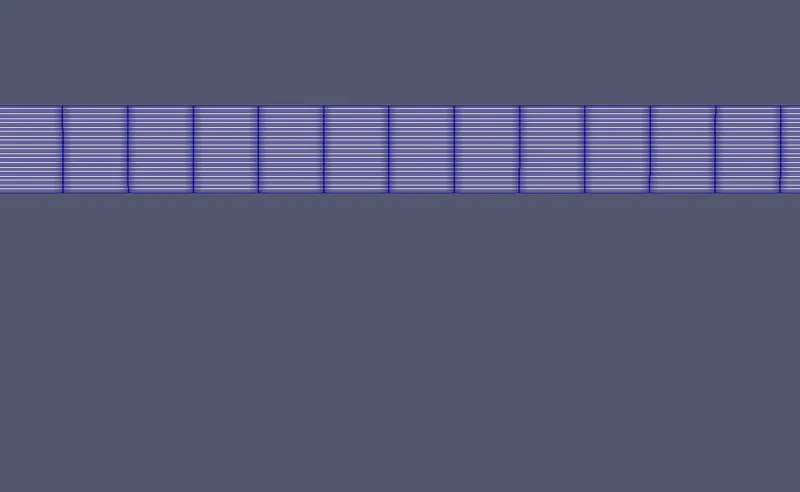
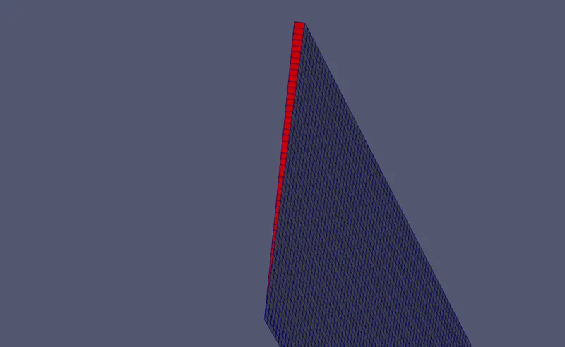
- Meshing results
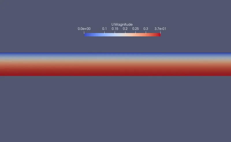
- Velocity contour
The image below shows the velocity profile at x = 0.75m from inlet
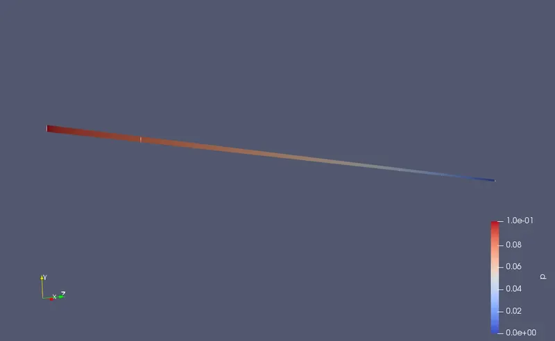
- Pressure Contour
- Velocity profile at different locations
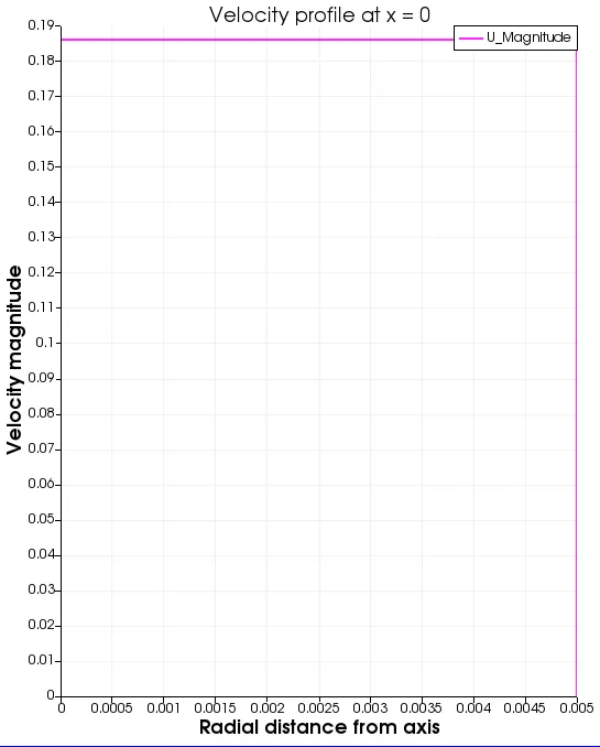
At the inlet (x=0) the flow is completely under developed and it can be seen through the velocity profile below.
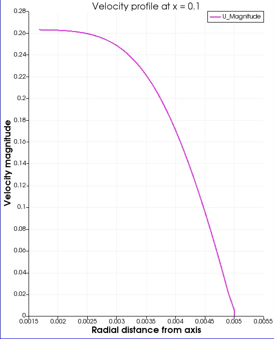
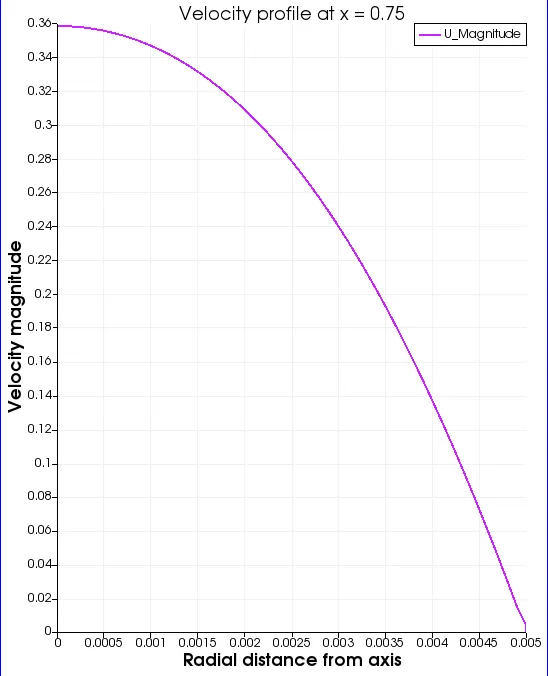
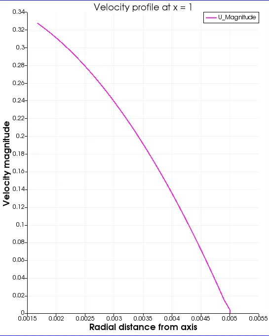
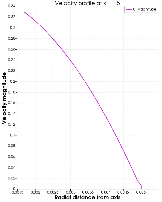
Considering the above three graphs (x=0.1;0.75 and 1), we can see that the velocity profile keeps changing. That means the flow still under developed. But from x = 0.75 to x = 1 we have a developing velocity profile which. According to the Hydrodynamic entrance length, the fully developed region starts at x = 1.26m . Hence we can see in the figure below (x=1.5m) the flow is fully developped.
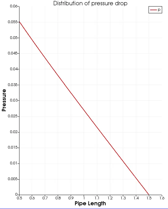
The above graph shows the pressure drop across the entire pipe.
Comparison of above results with Analytical solution Hagen poiseuille's equation
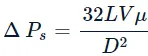
It is known as Hagen Poiseuille Equation and can be used to measure the viscosity of the fluid given its pressure drop and volumetric flow rate of a tub of a given diameter and length. As far as our problem is concerned, we will use it to calculate pressure drop of the fluid flow across the considered pipe.
Thus,

The maximum velocity is computed using the average velocity:

The results obtained from simulation are as follows:
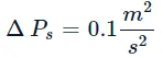
&
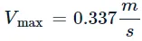
Hence we conclude that simulation results and analytical results matches closely or are quite the same.