To simulate an axi-symmetric flow by applying the wedge boundary condition. The flow is laminar and flows through a constant cross-section pipe at an inlet Reynold's number of 2100. You can do a transient or steady state simulation and have to validate results with the Hagen- Poiseuille's equations for the fully developed flow.
The Hagen-Poiseuille equation, also known as Poiseuille's law, describes the flow of a viscous fluid through a cylindrical pipe or tube. It relates the flow rate of the fluid to various parameters such as the pressure difference across the pipe, the pipe length, the pipe radius, and the viscosity of the fluid. The equation is named after Gotthilf Hagen and Jean Léonard Marie Poiseuille, who independently derived it.
where: Q is the volumetric flow rate of the fluid, ΔP is the pressure difference across the pipe, r is the radius of the pipe, η is the dynamic viscosity of the fluid, and L is the length of the pipe.
The equation shows that the flow rate (Q) is directly proportional to the pressure difference (ΔP) and the fourth power of the pipe radius (r^4), while it is inversely proportional to the viscosity (η) and the length of the pipe (L).
The Hagen-Poiseuille equation assumes laminar flow, where the fluid flows smoothly in parallel layers with no turbulence. It also assumes that the fluid is incompressible and the pipe has a constant circular cross-section.
This equation finds applications in various fields such as fluid dynamics, engineering, and medicine, where the flow of fluids through pipes or blood vessels needs to be analyzed or controlled.
for creating blockmesh we need to write code in matlab .Here for solving the problem numerically we will use the icoFoam solver with the cavity tutorial make the geometry along with the mesh and make the blockmeshDict file with the help of matlab as shown below:
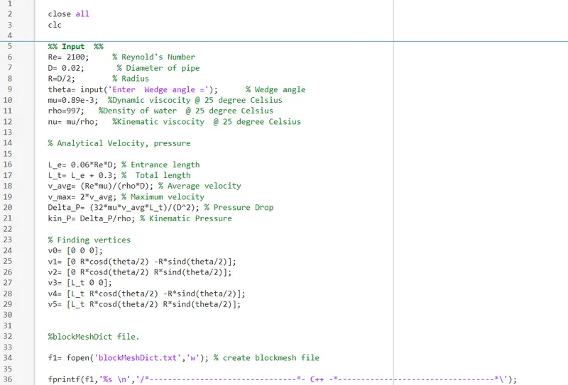
close all
clc
%% Input %%
Re= 2100; % Reynold's Number
D= 0.02; % Diameter of pipe
R=D/2; % Radius
theta= input('Enter Wedge angle ='); % Wedge angle
mu=0.89e-3; %Dynamic viscocity @ 25 degree Celsius
rho=997; %Density of water @ 25 degree Celsius
nu= mu/rho; %Kinematic viscocity @ 25 degree Celsius
% Analytical Velocity, pressure
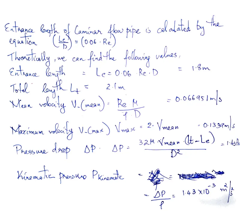
L_e= 0.06*Re*D; % Entrance length
L_t= L_e + 0.3; % Total length
v_avg= (Re*mu)/(rho*D); % Average velocity
v_max= 2*v_avg; % Maximum velocity
Delta_P= (32*mu*v_avg*L_t)/(D^2); % Pressure Drop
kin_P= Delta_P/rho; % Kinematic Pressure
% Finding vertices
v0= [0 0 0];
v1= [0 R*cosd(theta/2) -R*sind(theta/2)];
v2= [0 R*cosd(theta/2) R*sind(theta/2)];
v3= [L_t 0 0];
v4= [L_t R*cosd(theta/2) -R*sind(theta/2)];
v5= [L_t R*cosd(theta/2) R*sind(theta/2)];
%blockMeshDict file.
f1= fopen('blockMeshDict.txt','w'); % create blockmesh file
fprintf(f1,'%s \n','/*--------------------------------*- C++ -*----------------------------------*\');
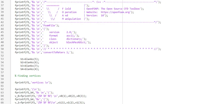
fprintf(f1,'%s \n',' ========= |');
fprintf(f1,'%s \n',' \\ / F ield | OpenFOAM: The Open Source CFD Toolbox');
fprintf(f1,'%s \n',' \\ / O peration | Website: https://openfoam.org');
fprintf(f1,'%s \n',' \\ / A nd | Version: 10');
fprintf(f1,'%s \n',' \\/ M anipulation |');
fprintf(f1,'%s \n','\*---------------------------------------------------------------------------*/');
fprintf(f1,'%s \n','FoamFile');
fprintf(f1,'%s \n','{');
fprintf(f1,'%s \n',' version 2.0;');
fprintf(f1,'%s \n',' format ascii;');
fprintf(f1,'%s \n',' class dictionary;');
fprintf(f1,'%s \n',' object blockMeshDict;');
fprintf(f1,'%s \n','}');
fprintf(f1,'%s \n','// * * * * * * * * * * * * * * * * * * * * * * * * * * * * * * * * * * * * * //');
fprintf(f1,'%s \n','convertToMeters 1;');
b1=blanks(5);
b2=blanks(6);
b3=blanks(7);
b4=blanks(4);
% Finding vertices
fprintf(f1,'vertices \n');
fprintf(f1,'(\n');
fprintf(f1,b4,'%s \n','(');
v_0=fprintf(f1,'(%f %f %f) \n',v0(1),v0(2),v0(3));
fprintf(f1,b4,'%s','(');
v_1=fprintf(f1,'(%f %f %f)\n',v1(1),v1(2),v1(3));
fprintf(f1,b4,'%s','(');
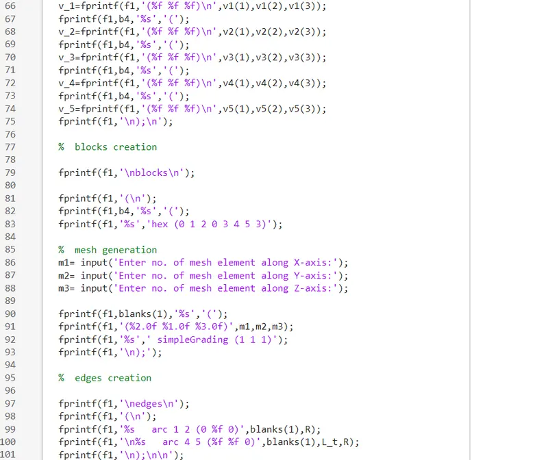
v_2=fprintf(f1,'(%f %f %f)\n',v2(1),v2(2),v2(3));
fprintf(f1,b4,'%s','(');
v_3=fprintf(f1,'(%f %f %f)\n',v3(1),v3(2),v3(3));
fprintf(f1,b4,'%s','(');
v_4=fprintf(f1,'(%f %f %f)\n',v4(1),v4(2),v4(3));
fprintf(f1,b4,'%s','(');
v_5=fprintf(f1,'(%f %f %f)\n',v5(1),v5(2),v5(3));
fprintf(f1,'\n);\n');
% blocks creation
fprintf(f1,'\nblocks\n');
fprintf(f1,'(\n');
fprintf(f1,b4,'%s','(');
fprintf(f1,'%s','hex (0 1 2 0 3 4 5 3)');
% mesh generation
m1= input('Enter no. of mesh element along X-axis:');
m2= input('Enter no. of mesh element along Y-axis:');
m3= input('Enter no. of mesh element along Z-axis:');
fprintf(f1,blanks(1),'%s','(');
fprintf(f1,'(%2.0f %1.0f %3.0f)',m1,m2,m3);
fprintf(f1,'%s',' simpleGrading (1 1 1)');
fprintf(f1,'\n);');
% edges creation
fprintf(f1,'\nedges\n');
fprintf(f1,'(\n');
fprintf(f1,'%s arc 1 2 (0 %f 0)',blanks(1),R);
fprintf(f1,'\n%s arc 4 5 (%f %f 0)',blanks(1),L_t,R);
fprintf(f1,'\n);\n\n');
% Apply boundary conditions
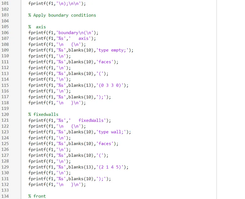
% axis
fprintf(f1,'boundary\n(\n');
fprintf(f1,'%s',' axis');
fprintf(f1,'\n {\n');
fprintf(f1,'%s',blanks(10),'type empty;');
fprintf(f1,'\n');
fprintf(f1,'%s',blanks(10),'faces');
fprintf(f1,'\n');
fprintf(f1,'%s',blanks(10),'(');
fprintf(f1,'\n');
fprintf(f1,'%s',blanks(13),'(0 3 3 0)');
fprintf(f1,'\n');
fprintf(f1,'%s',blanks(10),');');
fprintf(f1,'\n }\n');
% fixedwalls
fprintf(f1,'%s',' fixedWalls');
fprintf(f1,'\n {\n');
fprintf(f1,'%s',blanks(10),'type wall;');
fprintf(f1,'\n');
fprintf(f1,'%s',blanks(10),'faces');
fprintf(f1,'\n');
fprintf(f1,'%s',blanks(10),'(');
fprintf(f1,'\n');
fprintf(f1,'%s',blanks(13),'(2 1 4 5)');
fprintf(f1,'\n');
fprintf(f1,'%s',blanks(10),');');
fprintf(f1,'\n }\n');
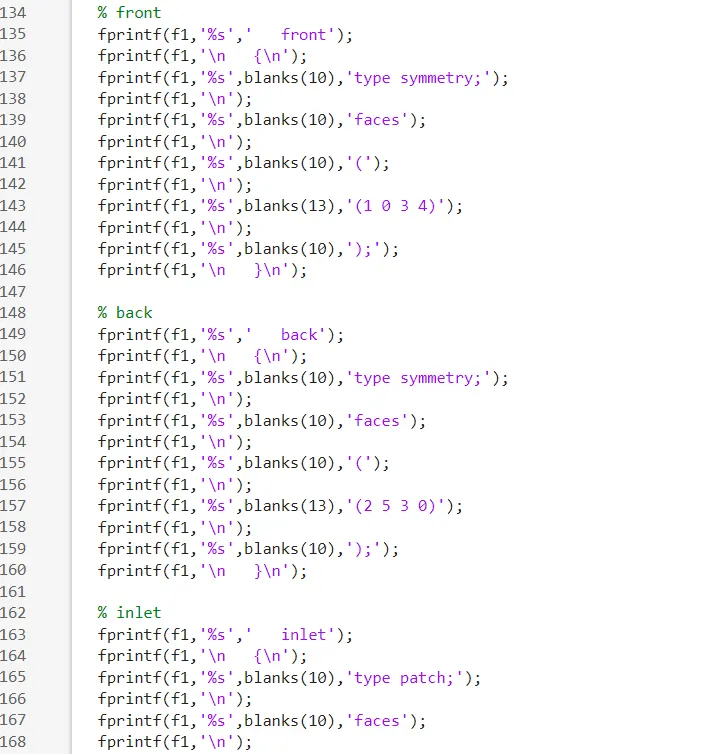
% front
fprintf(f1,'%s',' front');
fprintf(f1,'\n {\n');
fprintf(f1,'%s',blanks(10),'type symmetry;');
fprintf(f1,'\n');
fprintf(f1,'%s',blanks(10),'faces');
fprintf(f1,'\n');
fprintf(f1,'%s',blanks(10),'(');
fprintf(f1,'\n');
fprintf(f1,'%s',blanks(13),'(1 0 3 4)');
fprintf(f1,'\n');
fprintf(f1,'%s',blanks(10),');');
fprintf(f1,'\n }\n');
% back
fprintf(f1,'%s',' back');
fprintf(f1,'\n {\n');
fprintf(f1,'%s',blanks(10),'type symmetry;');
fprintf(f1,'\n');
fprintf(f1,'%s',blanks(10),'faces');
fprintf(f1,'\n');
fprintf(f1,'%s',blanks(10),'(');
fprintf(f1,'\n');
fprintf(f1,'%s',blanks(13),'(2 5 3 0)');
fprintf(f1,'\n');
fprintf(f1,'%s',blanks(10),');');
fprintf(f1,'\n }\n');
% inlet
fprintf(f1,'%s',' inlet');
fprintf(f1,'\n {\n');
fprintf(f1,'%s',blanks(10),'type patch;');
fprintf(f1,'\n');
fprintf(f1,'%s',blanks(10),'faces');
fprintf(f1,'\n');
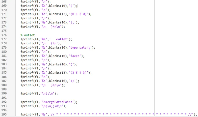
fprintf(f1,'%s',blanks(10),'(');
fprintf(f1,'\n');
fprintf(f1,'%s',blanks(13),'(0 1 2 0)');
fprintf(f1,'\n');
fprintf(f1,'%s',blanks(10),');');
fprintf(f1,'\n }\n\n');
% outlet
fprintf(f1,'%s',' outlet');
fprintf(f1,'\n {\n');
fprintf(f1,'%s',blanks(10),'type patch;');
fprintf(f1,'\n');
fprintf(f1,'%s',blanks(10),'faces');
fprintf(f1,'\n');
fprintf(f1,'%s',blanks(10),'(');
fprintf(f1,'\n');
fprintf(f1,'%s',blanks(13),'(3 5 4 3)');
fprintf(f1,'\n');
fprintf(f1,'%s',blanks(10),');');
fprintf(f1,'\n }\n\n');
fprintf(f1,'\n);\n');
fprintf(f1,'\nmergePatchPairs');
fprintf(f1,'\n(\n);\n\n');
fprintf(f1,'%s','// * * * * * * * * * * * * * * * * * * * * * * * * * * * * * * * * * * * * * //');
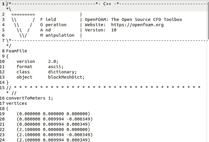
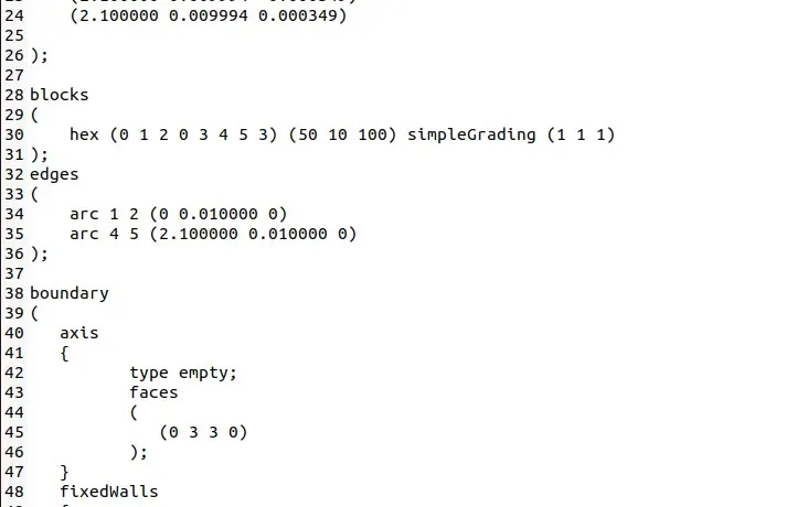
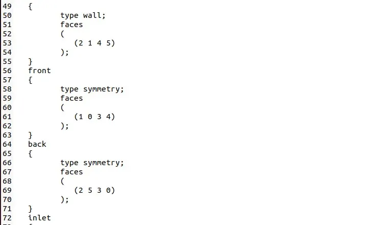
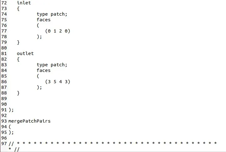
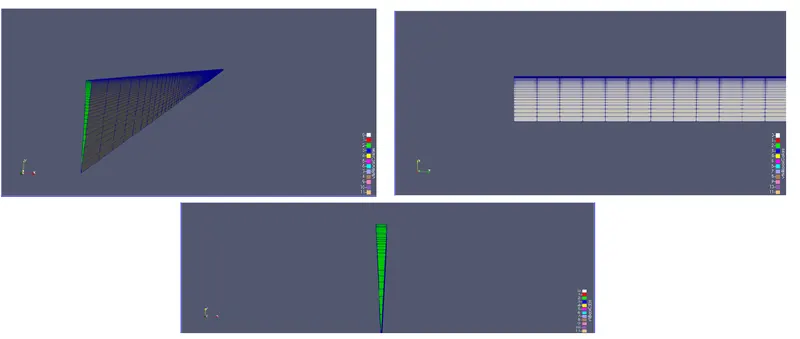
This is the blockmesh file created by the matlab code above
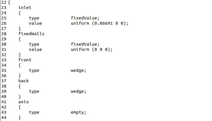
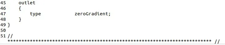
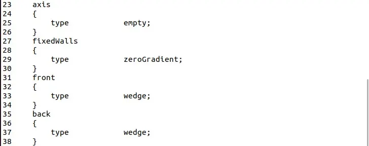
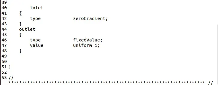
boundary condition
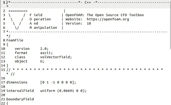
velocity file U which is in 0 directory .
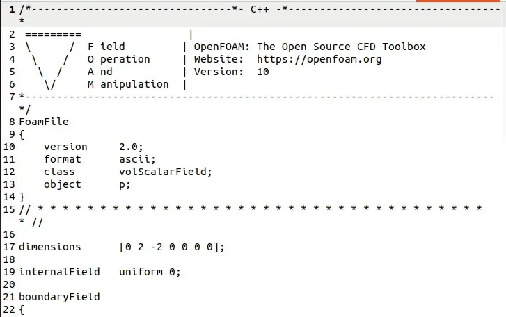
pressure file p
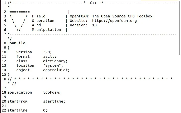
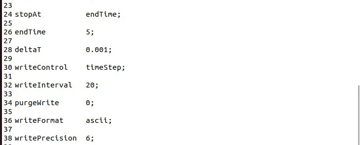
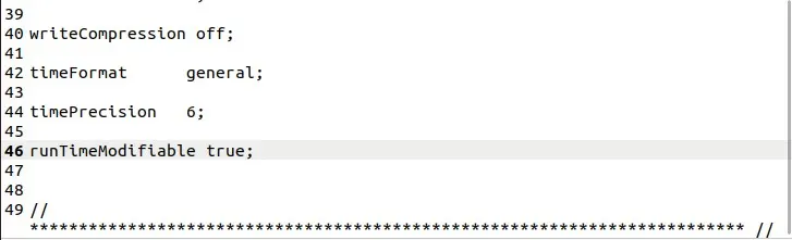
controDict file
result
geometry created is a wedge with 4 degree.
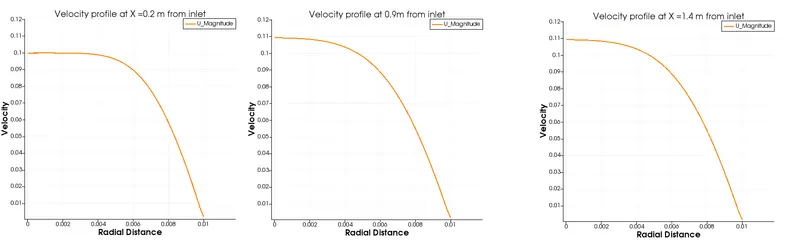
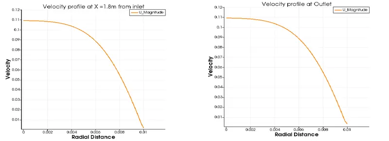
velocity plots at various regions
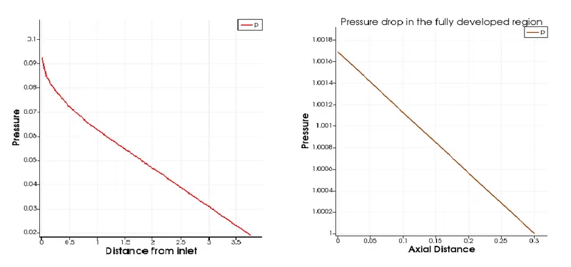
pressure profile
conclusion
After 1.8 m we can see the flow getting stable which means the flow is fully stable.
It is observed that the velocity profile gradually increased from inlet to the outlet. The velocity profile is observed to increase slowly at different lengths of pipe and also it reached maximum velocity at the outlet. This region is called as a fully developed region as the velocity profile completely developes at the outlet.
When the fluid is moving, shear stresses are developed as the particles in the flow move relative to each other. For a fluif flowing in a pipe, the fluid velocity remains zero at the pipe wall. Shear force is generated because of the adjacent layer of the fluid that move with different velocities. At the walls the velocity remains zero as we considered no slip boundary conditions. As the flowflow progress-gradually the boundary layers developand the adjacent layers tend to slow down. Because of this the velocity at the center increases. Hence, because of the pressure difference obtained from the equations, the velocity profile obayes Hagen Poiseuille's equation. Hence velocity profile matches with the Hagen poiseuille's equation.
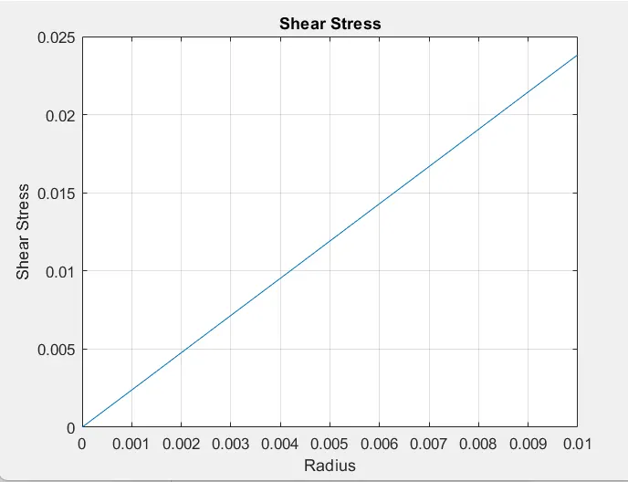
shear stress
Shear stress: It is the rate of change of velocity at which one layer of fluid passes over adjacent layer.
Formula
τ=μ(dudy)">τ= = μ ( d u)/ (d y )
This formula is applicable for newtonian fluids/ Laminar flow.
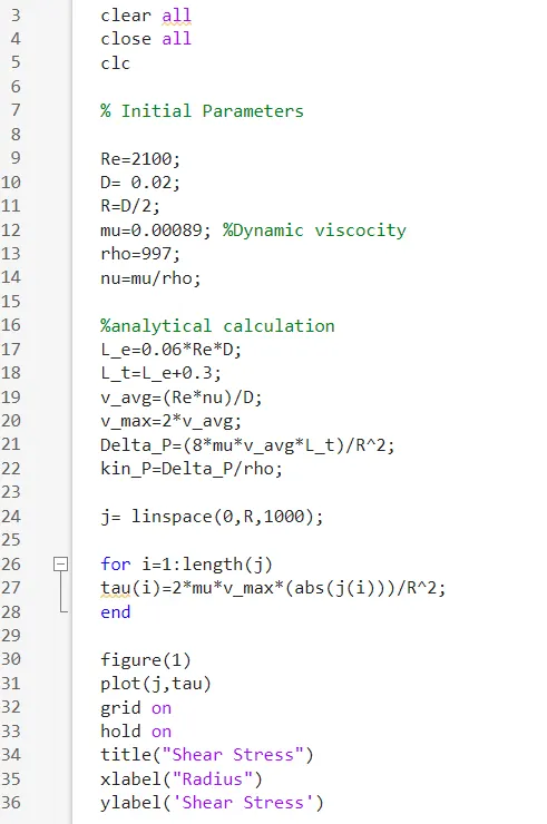
matlab code
clear all
close all
clc`τ = μ (( d u)/ (d y ))`
% Initial Parameters
Re=2100;
D= 0.02;
R=D/2;
mu=0.00089; %Dynamic viscocity
rho=997;
nu=mu/rho;
%analytical calculation
L_e=0.06*Re*D;
L_t=L_e+0.3;
v_avg=(Re*nu)/D;
v_max=2*v_avg;
Delta_P=(8*mu*v_avg*L_t)/R^2;
kin_P=Delta_P/rho;
j= linspace(0,R,1000);
for i=1:length(j)
tau(i)=2*mu*v_max*(abs(j(i)))/R^2;
end
figure(1)
plot(j,tau)
grid on
hold on
title("Shear Stress")
xlabel("Radius")
ylabel('Shear Stress')