Week 11 - Simulation of Flow through a pipe in OpenFoam
AIM
To simulate an axi-symmetric flow by applying the wedge boundary condition.
Expected Results
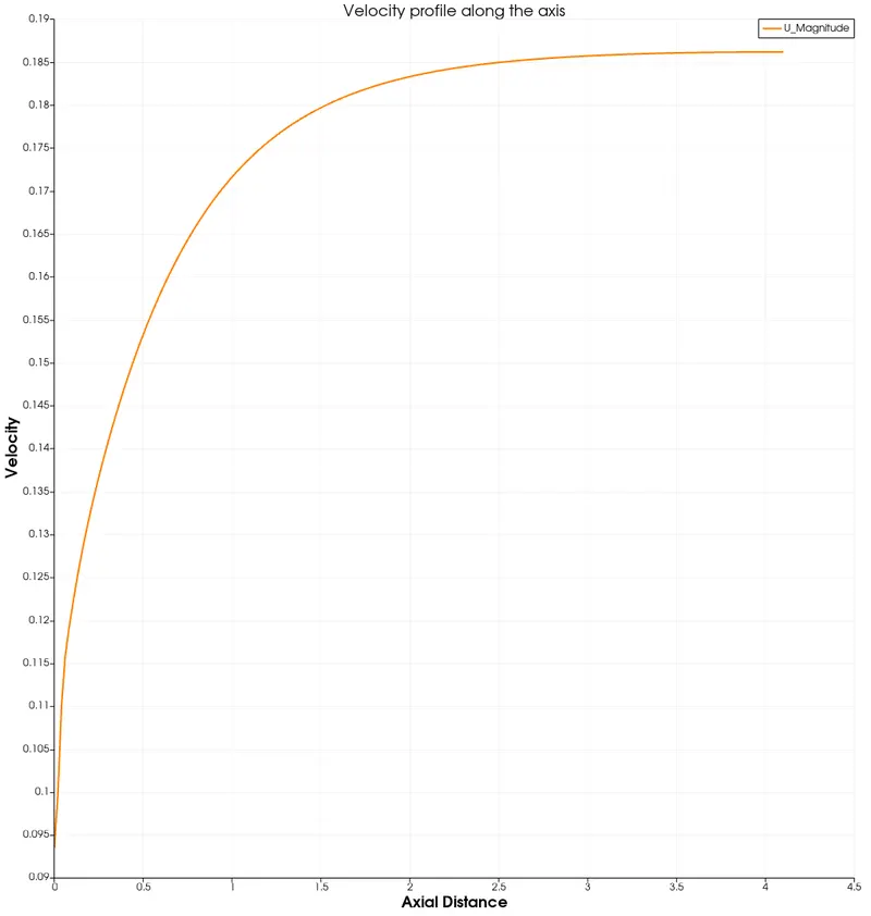
- Validate Hydro-dynamic length with the numerical result
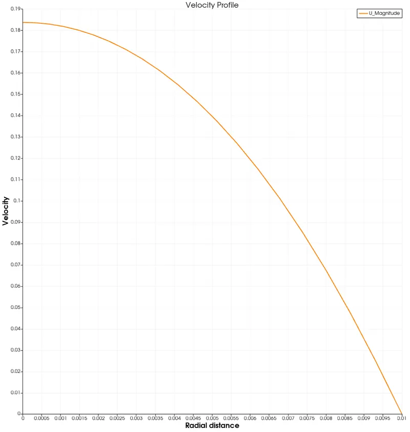
- Validate the fully developed flow velocity profile with its analytical profile
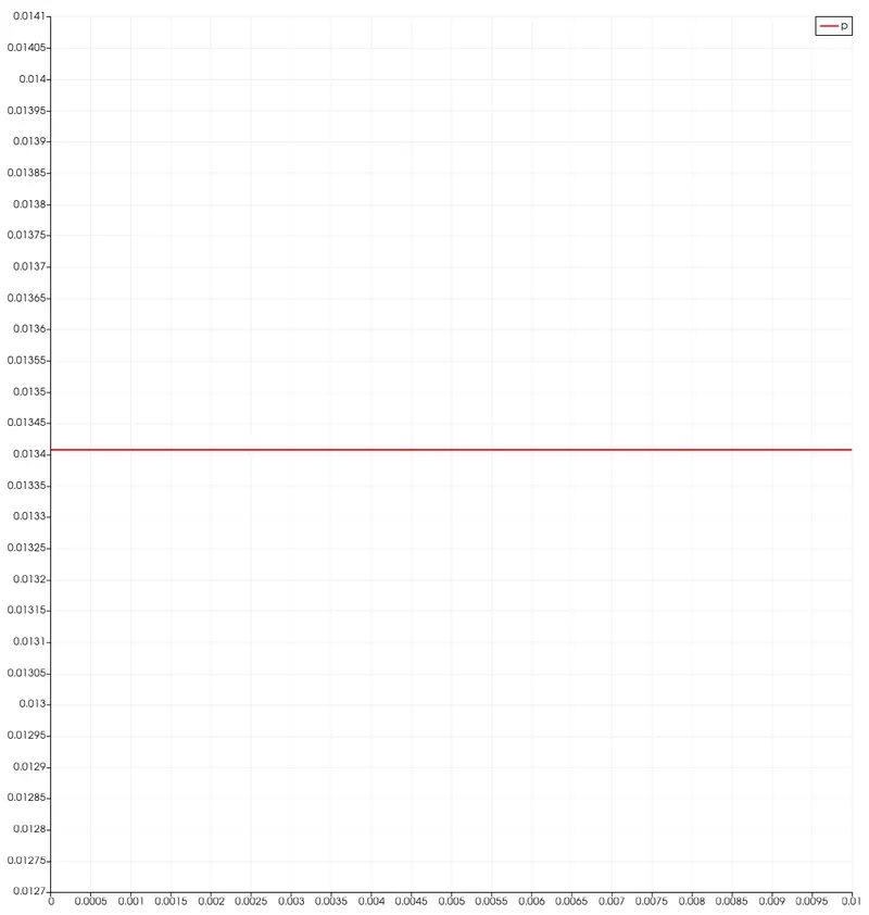
- Validate maximum velocity and pressured drop for fully developed flow
- Post-process Shear stress and validate wall shear stress for fully developed flow
THEORY
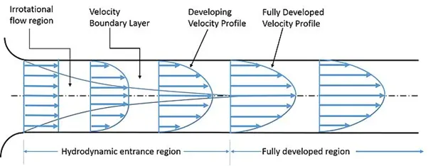
- The region of the flow in which the effects of the viscous shearing forces
caused by fluid viscosity are felt is called the velocity boundary layer or
just the boundary layer. - The hypothetical boundary surface divides the
flow in a pipe into two regions: the boundary layer region, in which the
viscous effects and the velocity changes are significant, and the irrotational
(core) flow region, in which the frictional effects are negligible and the
velocity remains essentially constant in the radial direction. - The thickness of this boundary layer increases in the flow direction until the boundary layer reaches the pipe center and thus fills the entire pipe and the velocity becomes fully developed a little farther
downstream. - The region from the pipe inlet to the point at which the velocity profile is fully developed is called the hydrodynamic entrance region,
and the length of this region is called the hydrodynamic entry length Lh.
Flow in the entrance region is called hydrodynamically developing flowsince this is the region where the velocity profile develops. - The region beyond the entrance region in which the velocity profile is fully developed
and remains unchanged is called the hydrodynamically fully developed
region. The flow is said to be fully developed when the normalized temperature profile remains unchanged as well
Hagen–Poiseuille law
For specified flow the flow rate, the pressure drops and thus the required pumping power is proportional to the length of the pipe and the viscosity of the fluid, but it is inversely
proportional to the fourth power of the radius (or diameter) of the pipe., is a physical law that gives the pressure drop in an incompressible and Newtonian fluid in laminar flow flowing through a long cylindrical pipe of constant cross section.
Hagen–Poiseuille equation
In standard fluid-kinetics notation.
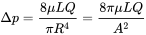
where:
- Δp is the pressure difference between the two ends,
- L is the length of pipe,
- μ is the dynamic viscosity,
- Q is the volumetric flow rate,
- R is the pipe radius,
- A is the cross section of pipe.
Given parameters
- Wedge angle less than 5 degrees,
- Flow is axi symetrical.
- Fluid is incompressible and the flow is laminar.
Expected Velocity Profile.
Assumptions
- The distance the fluid has to travel to become fully developed is given by the Entry Length formula.
- Given Reynolds number is 2100. This implies flow is laminar.
- Hence Entry length formula for Laminar is given by: Ld=0.06.Re">Ld=0.06.ReLd=0.06.Re
- where L is effective length; d is dia of pipe and Re is reyonolds number.
Steps
- We initialy created blockmeshDict file by means of matlab code
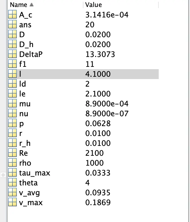
- In matlab code we calculated the total length of pipe ,average velocity ,maximum velocity,maximum shear stress and pressure drop using Hagen–Poiseuille equation
- Then we utilized this file to create mesh.
- Concept of mesh is that ,we take a wedge section of the pipe as flow region and we done analysis by this region
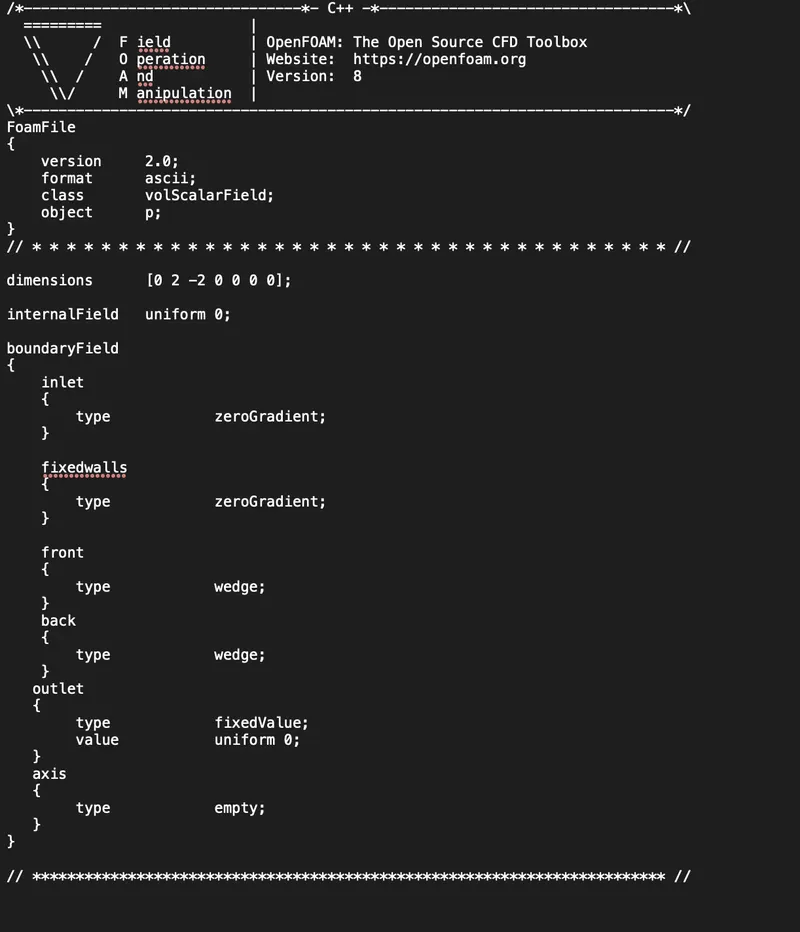
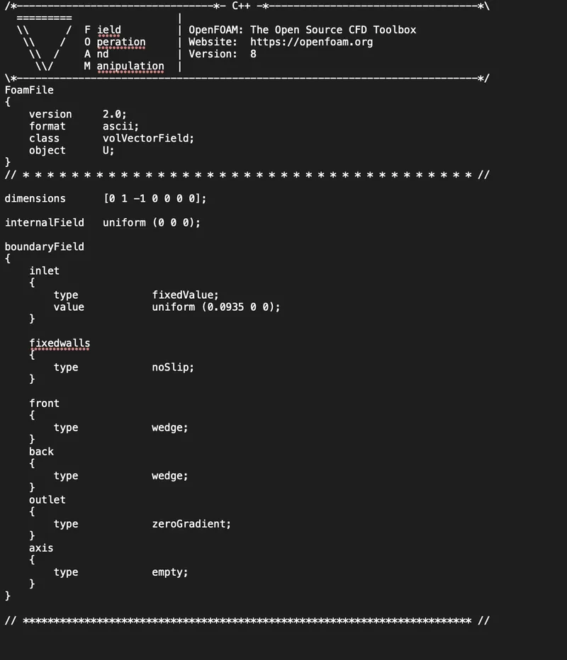
- The velocity and pressure bc are applied
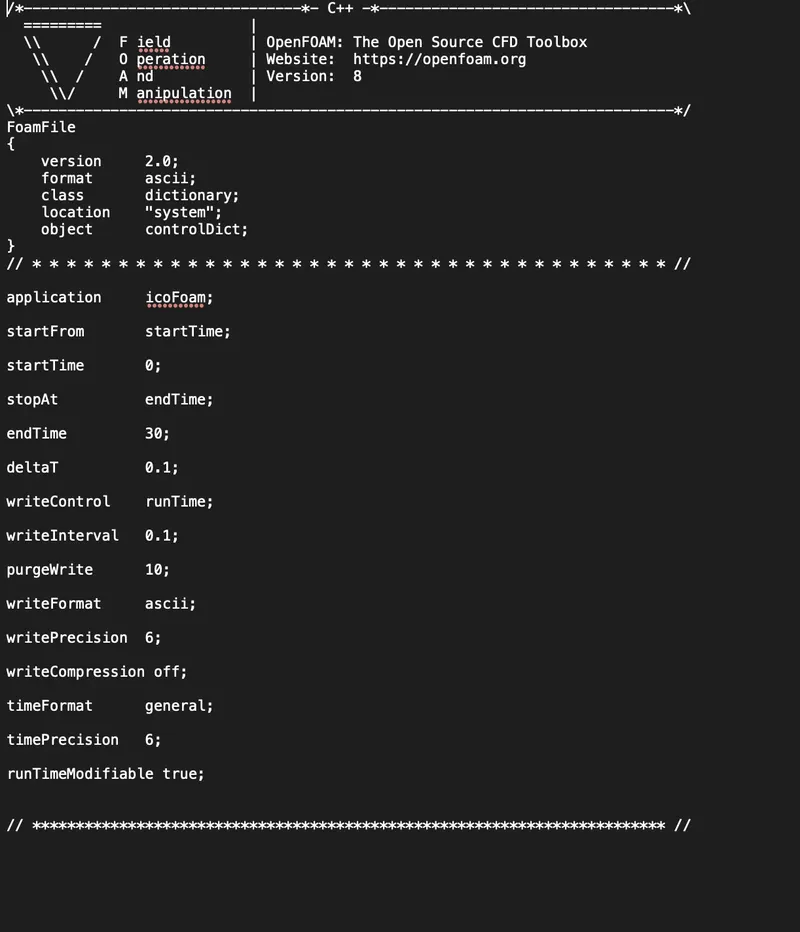
- The controlDict file is edited for Simulation run time and timestep;
- Then, the simulation started by calling 'icoFoam' command in the terminal.
- 'paraFoam' command helps to open paraView
- The shear stress diagram is obtained by post-processing the velocity results obtained from Openfoam.
icofoam solver
icoFoam solves the incompressible laminar Navier-Stokes equations using the PISO algorithm. The code is inherently transient, requiring an initial condition (such as zero velocity) and boundary conditions. The icoFOAM code can take mesh non-orthogonality into account with successive non-orthogonality iterations. The number of PISO corrections and non-orthogonality corrections are controlled through user input.
MATLAB CODE
clear all
close all
clc

Re = 2100; %Reynolds Number
rho = 1000; % Density
mu =  0.00089;
nu = mu/rho; %kinematic viscosity
ld=2 % length in m
D = 0.02;
r=D/2;% Dia of the pipe in meters
A_c = (pi/4)*D^2; % Cross sectional area
p = pi*D; % wetted perimeter
D_h = 4*A_c/p; %-> Hydraulic Dia of pipe
r_h = D_h/2; %Hydralic radius of pipe
theta=4;
v_avg = (Re*mu)/(rho*D_h);% Avg velocity
v_max = 2*v_avg; %Fully developed V max
le = 0.05*Re*D;     % Hydro Dynamci entrance length
l = le+ld;  % Total length ofo the pipe
DeltaP = 32*mu*v_avg*ld/(D^2);
tau_max=2*mu*v_max/r_h;

f1=fopen('blockMeshDict','w')
fprintf(f1,'FoamFile\n{\n')
fprintf(f1,'version     2.0;\n')
fprintf(f1,'format      ascii;\n')
fprintf(f1,'class       dictionary;\n')
fprintf (f1,' object    blockMeshDict;\n}\n\n')
fprintf(f1,'convertToMeters 1;\n\n')
fprintf(f1,'vertices\n(\n')
fprintf(f1,'(%d %d %d)\n',0,0,0)                                  %0
fprintf(f1,'(%d %d %d)\n',0,(r*cosd(theta/2)),(r*sind(theta/2)))  %1
fprintf(f1,'(%d %d %d)\n',0,(r*cosd(theta/2)),(-r*sind(theta/2))) %3
fprintf(f1,'(%d %d %d)\n',l,0,0)                                  %4
fprintf(f1,'(%d %d %d)\n',l,(r*cosd(theta/2)),(r*sind(theta/2)))  %5
fprintf(f1,'(%d %d %d)\n);\n',l,(r*cosd(theta/2)),(-r*sind(theta/2))) %6
fprintf(f1,'blocks\n(\n')
fprintf(f1,'\thex')
fprintf(f1,'\t(%d %d %d %d %d %d %d %d)',0,3,5,2,0,3,4,1)
fprintf(f1,' (%d %d %d)',200,20,1)
fprintf(f1,'\tsimpleGrading (')
fprintf(f1,'%d %d %d)\n);\n',0,1,0)

fprintf(f1,'edges\n(\n')
fprintf(f1,'arc %d %d\t',1,2)
fprintf(f1,'(%d %d %d)\n',0,r,0)
fprintf(f1,'arc %d %d\t',4,5)
fprintf(f1,'(%d %d %d)\n);\n',l,r,0)
fprintf(f1,'boundary\n(\n')
fprintf(f1,'inlet\n{\n')
fprintf(f1,'\t type patch;\n')
fprintf(f1,'\t faces \n \t(\n')
fprintf(f1,'\t\t (%d %d %d %d)\n\t);\n}\n',0,1,2,0)
fprintf(f1,'fixedwalls\n{\n')
fprintf(f1,'\t type wall;\n')
fprintf(f1,'\t faces\n\t(\n')
fprintf(f1,'\t\t(%d %d %d %d)\n);\n}\n',1,4,5,2)
fprintf(f1,'front\n{\n')
fprintf(f1,'\t type wedge;\n')
fprintf(f1,'\t faces\n\t(\n')
fprintf(f1,'\t\t(%d %d %d %d)\n);\n}\n',0,3,4,1)
fprintf(f1,'back \n{\n')
fprintf(f1,'\t type wedge;\n')
fprintf(f1,'\t faces\n\t(\n')
fprintf(f1,'\t\t(%d %d %d %d)\n);\n}\n',0,2,5,3)
fprintf(f1,'outlet\n{\n')
fprintf(f1,'\ttype patch;\n')
fprintf(f1,'\tfaces\n\t(\n')
fprintf(f1,'\t\t (%d %d %d %d)\n\t);\n}\n',3,5,4,3)
fprintf(f1,'axis\n{\n')
fprintf(f1,'\t type empty;\n\tfaces\n\t(\n')
fprintf(f1,'\t  (%d %d %d %d)\n);\n}\n',0,3,3,0)
fprintf(f1,'mergePatchPairs\n(\n);')
blockMeshDict
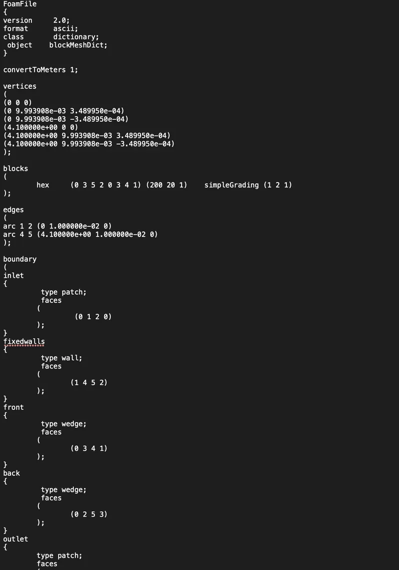
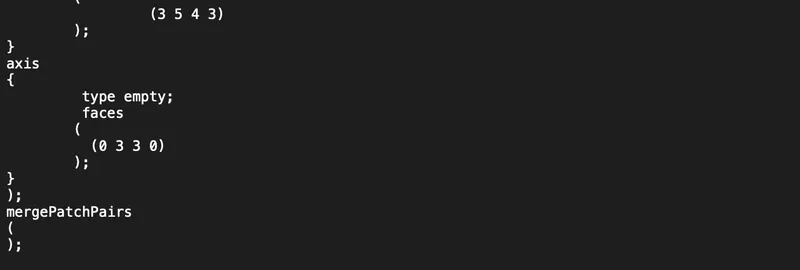
FoamFile
{
version     2.0;
format      ascii;
class       dictionary;
 object    blockMeshDict;
}

convertToMeters 1;

vertices
(
(0 0 0)
(0 9.993908e-03 3.489950e-04)
(0 9.993908e-03 -3.489950e-04)
(4.100000e+00 0 0)
(4.100000e+00 9.993908e-03 3.489950e-04)
(4.100000e+00 9.993908e-03 -3.489950e-04)
);

blocks
(
	hex	(0 3 5 2 0 3 4 1) (200 20 1)	simpleGrading (1 2 1)
);

edges
(
arc 1 2	(0 1.000000e-02 0)
arc 4 5	(4.100000e+00 1.000000e-02 0)
);

boundary
(
inlet
{
	 type patch;
	 faces
 	(
		 (0 1 2 0)
	);
}
fixedwalls
{
	 type wall;
	 faces
	(
		(1 4 5 2)
	);
}
front
{
	 type wedge;
	 faces
	(
		(0 3 4 1)
	);
}
back
{
	 type wedge;
	 faces
	(
		(0 2 5 3)
	);
}
outlet
{
	type patch;
	faces
	(
		 (3 5 4 3)
	);
}
axis
{
	 type empty;
	 faces
	(
	  (0 3 3 0)
	);
}
);
mergePatchPairs
(
);
controlDict
PRESSURE
VELOCITY
OUTPUTS
Output from matlab code
VELOCITY PROFILE
AXIAL VELOCITY PROFILE
SHEAR STRESS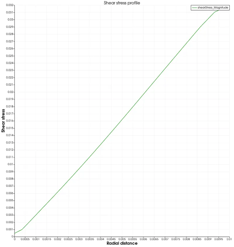
PRESSURE PROFILE
Observation
- From the plots we can see that for fully developed laminar flow, each fluid particle moves at a constant
axial velocity along a streamline and the velocity profile u remains
unchanged in the flow direction. - Also there is no pressure drop after after hydrodynamic entrance region
- There is no motion in the radial direction and thus the velocity component in the direction normal to flow is everywhere zero
| maximum velocity(m/s) | pressure loss(pa) | max.shear stress(pa) | ||
| Numerical results | 0.186 | 0.01867 | 0.033 | |
| Analytical results | 0.184 | 0.0186 | 0.032 |
CONCLUSION
- Simulation is done and results are satisfactory
- Understands the laminar flow and its boundary layer nature
- understands basics of openfoam
all files is attached below