Week 11 - Simulation of Flow through a pipe in OpenFoam
AIM:
The object of the report is to perform simulation of flow through a pipe in OpenFOAM and validate the results.
THEORY:
In nonideal fluid mechanics, the Hagen-Poiseuille equation is also known as Hagen-Poiseuille law. In Haigen-Poiseuille flow, a Newtonian fluid is flowing through a long pipe with a constant cross-section area. Poiseuille's Equation describes the pressure drop due to the viscosity of the fluid.
The Hagen–Poiseuille equation can be derived from the Navier-Stokes equations. The laminar flow through a pipe of uniform circular cross-section is known as Hagen–Poiseuille flow. The equations governing the Hagen–Poiseuille flow can be derived directly from the Navier-Stokes momentum equations in 3D cylindrical coordinates (r, θ, x)
Assumptions -
- The flow is steady (∂ϕ/∂t = 0), where ϕ is the field variable
- The radial and azimuthal components of the fluid velocity are zero (vr = vθ = 0)
- The flow is axisymmetric (∂ϕ/∂θ = 0)
- The flow is fully developed (∂vx/∂x = 0)
The velocity vector in 3D-cylindrical system can be written as

From the assumptions, V = Vx ------------------------------------------------------(1)
The axial momentum equation is reduced to
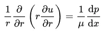 -----------------------------------------------------(2)
The radial momentum equation is reduced to
 -----------------------------------------------------------------------(3)
Diagramatic representation of velocity profile -
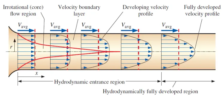
In, Haigen–Poiseuille flow the flow is laminar (Re < 2100). The entire domain is divided into - (1) Hydrodynamic entrance region (2) Hydrodynamically fully developed region.
Due to no-slip wall boundary conditions, the fluid velocity near the walls decreases and due to viscosity the adjacent fluid layers also decreases its velocity. So, in hydrodynamic entrance region, the fluid flow is continuously changing and in fully developed regions the flow becomes stable.
NOTE - Since, Haigen-Poiseuille assumed fully developed flow, the equations are derived for fully developed region only.
Fully developed region -
From eq - 1,2,3, by applying boundary conditions
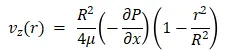 -----------------------------------------------------------------------(4)
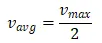 ------------------------------------------------------------------------------------------(5)
 ---------------------------------------------------------------------------------------(6)
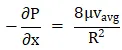
Therefore, in fully developed region, the velocity profile is parabolic and there is a constant pressure drop across the length of the cylinder. The eq (6) represents the pressure difference between the inlet and outlet of the pipe in order for the viscous Newtonian fluid to flow through the pipe.
PROBLEM STATEMENT -
Consider, working fluid as water.
Given, Reynoulds number (Re) = 2100
Dynamic viscosity = 1e-3 pa-s
Density = 1000 kg/m3
kinematic viscosity(nu) = 1e-6 m2/s
Assume, the diameter of pipe (D) = 0.1m.
The hydrodynamic entry length L(h,laminar) = 0.0575*Re*D = 12.075 m.
So, the total length of pipe is considered as L = 15 m.
Inlet velcotiy is calculated from reynoulds number i.e, V = Re*(nu)/D = 0.021 m/s
PROCEDURE :
Perform the simulation by using OpenFoam software. From the assumptions taken above, as the flow is axi-symmetrical.
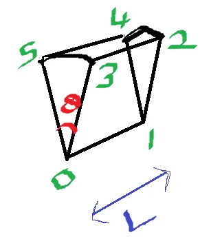
Since, in axi-symmetry flow the results can be mirrored, instead of performing simulation to the entire pipe, a sector of wedge angle < 5degrees is considered so that the computational cost is reduced.
Wedge angle (θ) = 3 degrees
The following fig shows the wedge block that is to be modelled.
STEP 1 - Writing blockMeshDict file in matlab
Re = 2100; %%reynoulds number
D = 0.1; %%diameter of pipe in meters
R = D/2; %%radius in meters
Le = 0.0575*Re*D; %%entry length
L = 15; %%length of pipe

mu = 1e-3; %%dynamic viscosity (kg/m^3)
rho = 1e3; %%density (m^2/s)
nu = mu/rho; %%kinematic viscosity
u = 0.021; %%inlet velocity (m/s)
theta = 3; %%degrees


%%verices
v0 = [0 0 0];
v1 = [0 0 -L];
v2 = [R*sind(theta/2) R*cosd(theta/2) -L];
v3 = [R*sind(theta/2) R*cosd(theta/2) 0];
v4 = [-R*sind(theta/2) R*cosd(theta/2) -L];
v5 = [-R*sind(theta/2) R*cosd(theta/2) 0];

%grid descretization
n1 = 50;
n2 = 1;
n3 = 2000;
n = [50 1 2000];

%simple grading
s1 = 0.2;
s2 = 1;
s3 = 1;
s = [0.2 1 1];


f1 = fopen('blockMeshDict.txt','w')
fprintf(f1,'FoamFile\n{\n')
fprintf(f1,'\tformat \t ascii;\n')
fprintf(f1,'\tclass \t dictionary;\n')
fprintf(f1,'\tobject \t blockMeshDict;\n}\n')
fprintf(f1,'\n//*******************************//\n\n')
fprintf(f1,'convertToMeters 1')
fprintf(f1,'\n\n')
fprintf(f1,'vertices\n{')
fprintf(f1,'\n\t (%d %d %d)',v0)
fprintf(f1,'\n\t (%d %d %d)',v1)
fprintf(f1,'\n\t (%7.6d %7.6d %d)',v2)
fprintf(f1,'\n\t (%7.6d %7.6d %d)',v3)
fprintf(f1,'\n\t (%7.6d %7.6d %d)',v4)
fprintf(f1,'\n\t (%7.6d %7.6d %d) \n};',v5)
fprintf(f1,'\nblocks\n(')
fprintf(f1,'\t hex (0 5 3 0 1 4 2 1)')
fprintf(f1,' (%d %d %d) %s (%2d %d %d) \n);',n,'simpleGrading',s)
fprintf(f1,'\nedges \n(')
fprintf(f1,'\tarc 5 3 (%d %2.1d %d)\n',0,R,0)
fprintf(f1,'\tarc 4 2 (%d %2.1d %d)\n',0,R,-L)
fprintf(f1,'\nboundary \n(')
fprintf(f1,'\n\tinlet \n\t{ \n\t\ttype patch; \n\t\tfaces \n\t\t( \n\t\t\t(0 3 5 0) \n\t\t); \n\t}')
fprintf(f1,'\n\toutlet \n\t{ \n\t\ttype patch; \n\t\tfaces \n\t\t( \n\t\t\t(1 4 2 1) \n\t\t); \n\t}')
fprintf(f1,'\n\tfixedWalls \n\t{ \n\t\ttype wall; \n\t\tfaces \n\t\t( \n\t\t\t(3 2 4 5) \n\t\t); \n\t}')
fprintf(f1,'\n\tfront \n\t{ \n\t\ttype wedge; \n\t\tfaces \n\t\t( \n\t\t\t(0 1 2 3) \n\t\t); \n\t}')
fprintf(f1,'\n\tBack \n\t{ \n\t\ttype wedge; \n\t\tfaces \n\t\t( \n\t\t\t(0 5 4 1) \n\t\t); \n\t}')
fprintf(f1,'\n\taxis \n\t{ \n\t\ttype empty; \n\t\tfaces \n\t\t( \n\t\t\t(0 1 1 0) \n\t\t); \n\t}\n);')
fprintf(f1,'\nmergedPatchPairs \n( \n); \n\n// ************************************************//')
fclose(f1)
STEP 2 - Pre-processing in OpenFoam
1)Generating mesh -
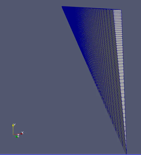
The block mesh is generated in blockMeshDict file. Import the blockmesh file generated by using matlab.
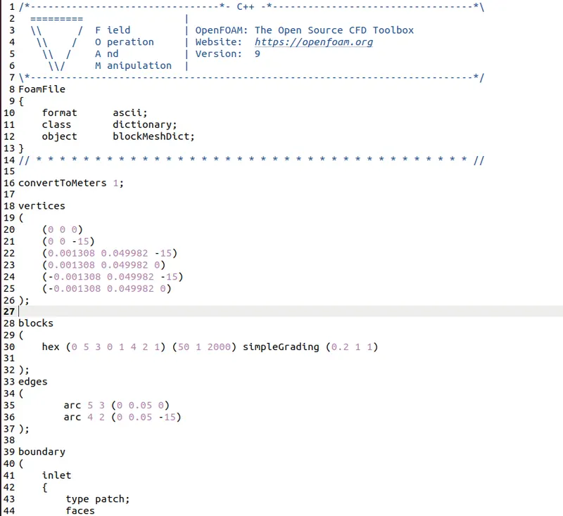
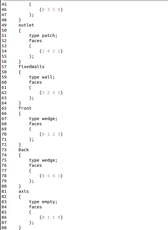

To generate mesh, type blockMesh in the terminal and the generated mesh is stored in the CONSTANT -> POLYMESH folder.
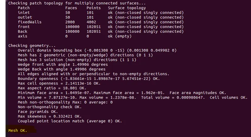
checkMesh command executes the quality of mesh. MESH OK in the fig indicates, there are no quality issues in the mesh.
Generated mesh in paraview
2) Initial and Boundary conditions -
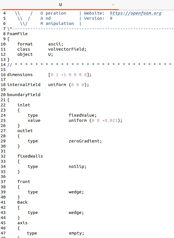
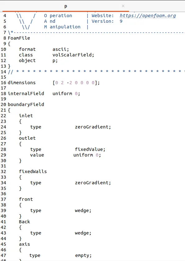
The initial and boundary conditions are present in the '0' folder. Input the values of velocity and pressure as per the requirements.
3) Control Dict -
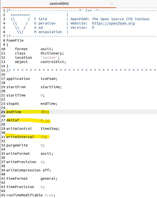
The ControlDict file present in the system folder. The controlDict file contains the necessary time inputs for the simulation.
NOTE- The time step (dt) should satisfy CFL criteria.
STEP 3 - Solving
After generating the mesh, simulate the model. Since, it is icofoam solver, type icoFoam in the terminal to perform simulation.
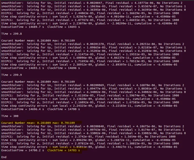
From the fig, the max courant number is 0.701. Since the courant number < 1, stable solution is obtained.
Total run time = 14703 sec = 4hr:5min
STEP 3 - Post processing
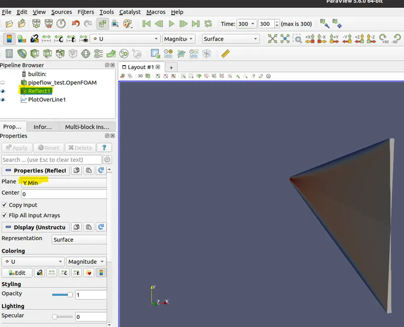
In command terminal, type paraFoam to open paraview tool. Since it is axisymmetric flow, the results are mirrored by FILTERS > ALPHABETICAL > REFLECT. Here, Ymin plane is the plane of reflection.
Fully developed region -
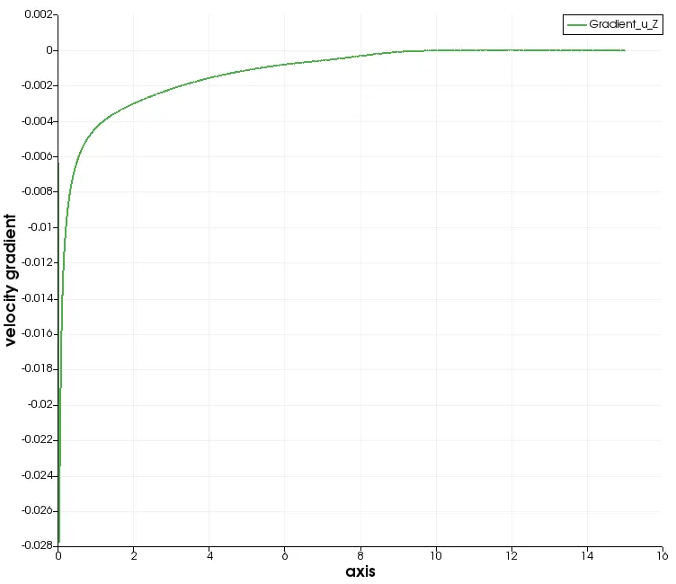
Hydrodynamic entry length (Le,h) = 0.0575*Re*D = 12.075m. The length of the pipe is 15m. So, fully developed flow is reached after 12.075m from inlet.
Condition for fully developed flow - du/dz = 0
So, form the plot it is observed that velocity gradient reaches to zero at z = 12m. Since, due to viscous effect the velocity decreases, negative velocity gradient is observed in the plot.
Field variables(velocity & pressure) plots at different time states -
The total termination time is 300sec. The following graphs shows the plots of velocity and kinematic pressure at time steps - 0 ,50 ,100, 200, 300.
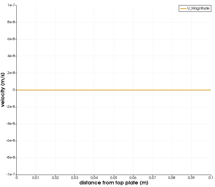
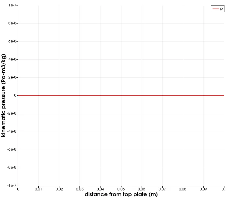
FIG - Plot at t =0sec at section 14m from inlet
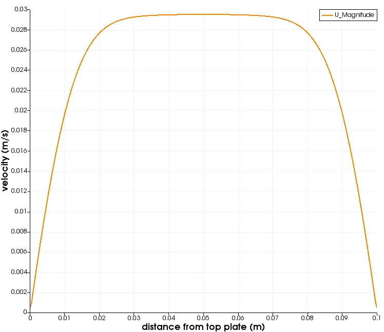
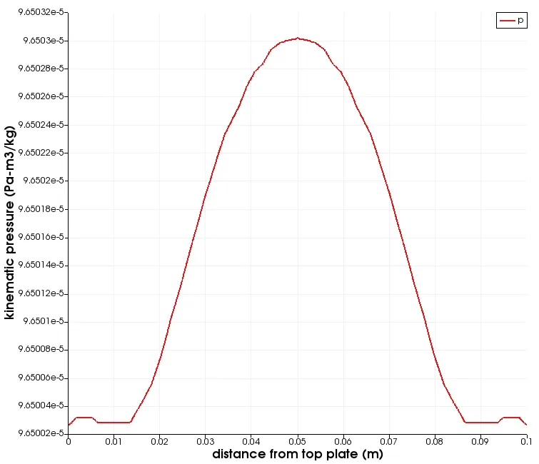
FIG - Plot at t =50sec at section 14m from inlet
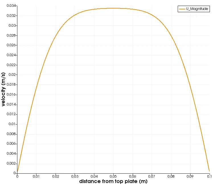
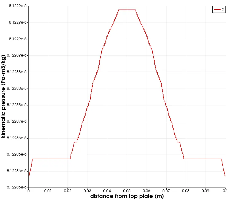
FIG - Plot at t =100sec at section 14m from inlet
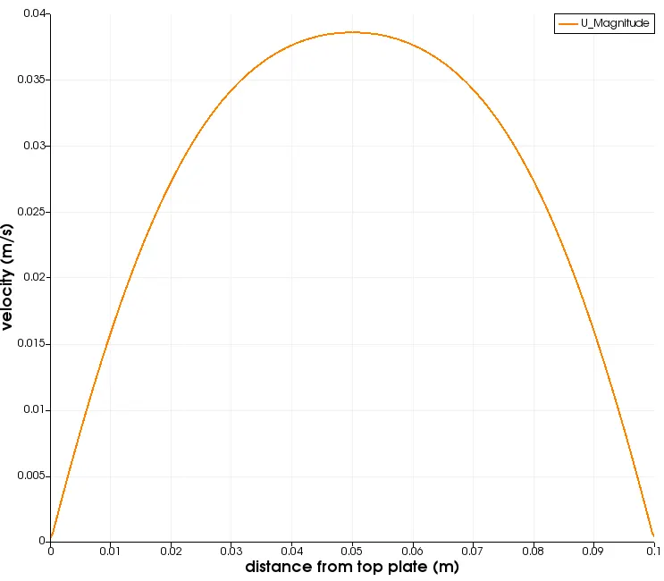
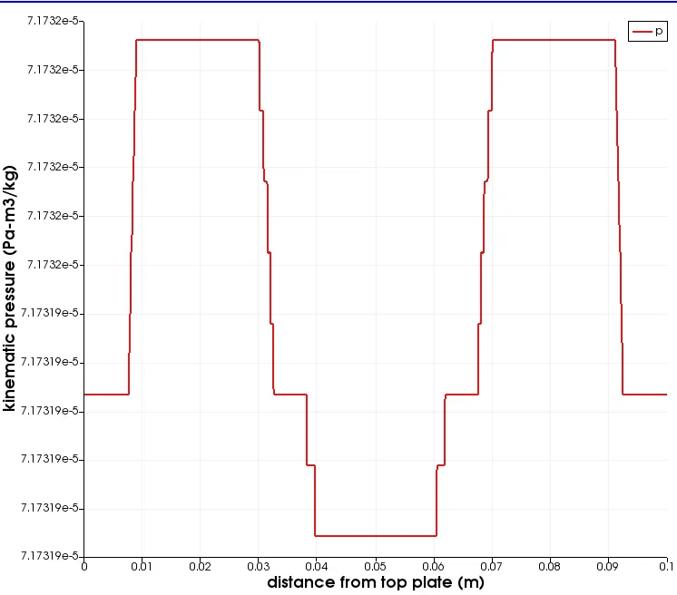
FIG - Plot at t =200sec at section 14m from inlet
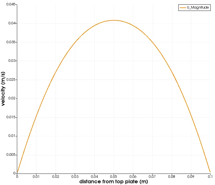
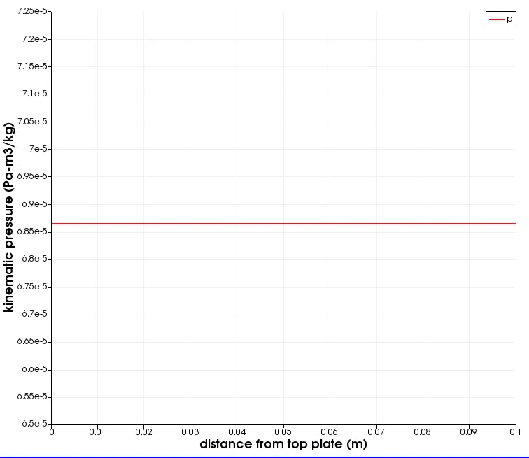
FIG - Plot at t =300sec at section 14m from inlet
NOTE - In fully developed flow, Velocity is parabolic profile and pressure gradient is zero across a section.
In the above plots, x = 0 indicates top surface of wedge
x = 0.1 indicates bottom surface of wedge
At, L = 12.075 m from inlet, fully developed flow exists. From the above fig, it is observed that at t = 300sec, the flow reaches steady state and fully developed flow is achieved. The max velocity exists at the center of the cylinder and is equal to around 0.042 m/s. Since in fully developed flow, there is zero pressure gradient along the radius, the kinematic pressure is constant across the section and is equal to 6.865e-5 Pa-m3/kg.
Velocity and pressure plot at steady steady (t = 300sec) over the entire domain -
In fully developed region, the velocity gradient along the length is zero. The following graphs shows the plots of velocity over the domain of the cylinder at L = 0, 2.5, 5, 10, 12, 14, 15 m from the inlet. From the plots, it is observed that After L = 12m, the flow reached a fully developed flow and the maximum velocity in fully developed region is v=0.042 m/s. The velocity profile is parabolic in a fully developed flow.
NOTE - Hagen-Poiseuille's in the derivation, assumed that in fully developed region, the pressure gradient is zero across a section.
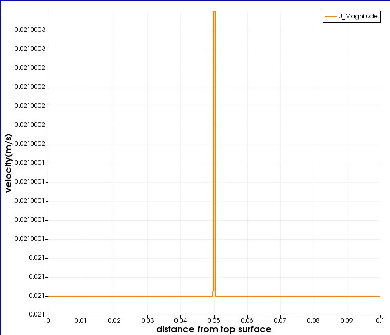
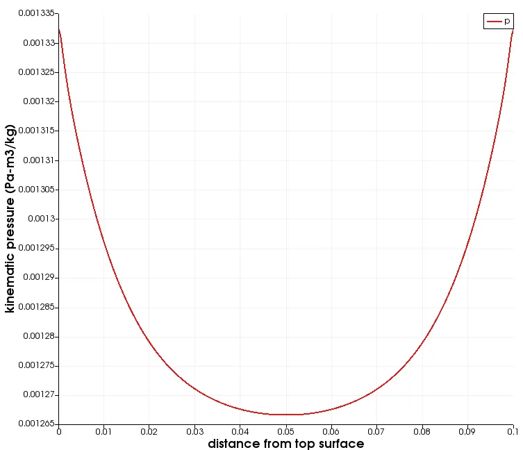
FIG - At t = 300sec, L = 0m from inlet
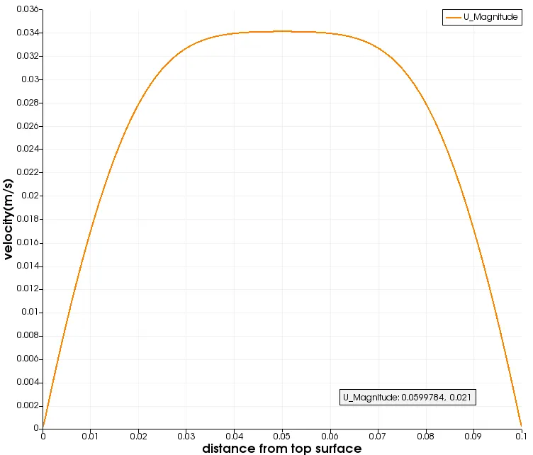
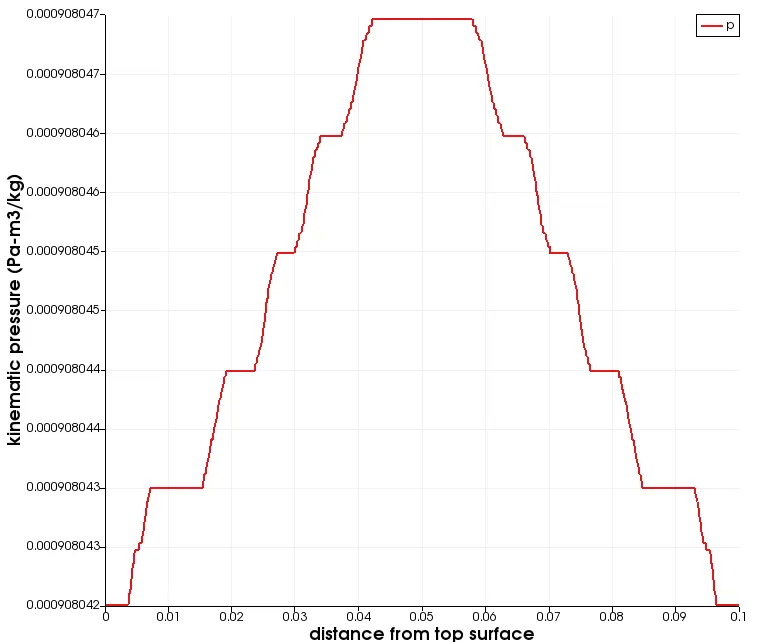
FIG - At t = 300sec, L = 2.5m from inlet
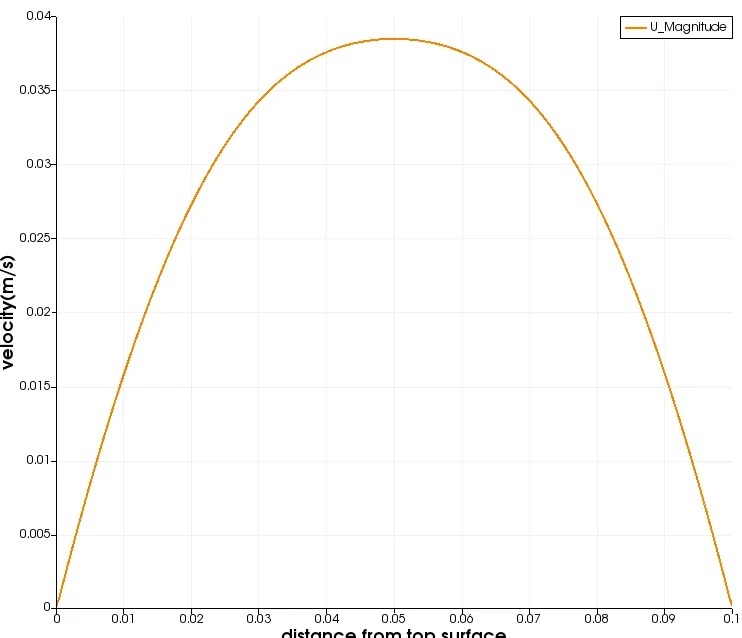
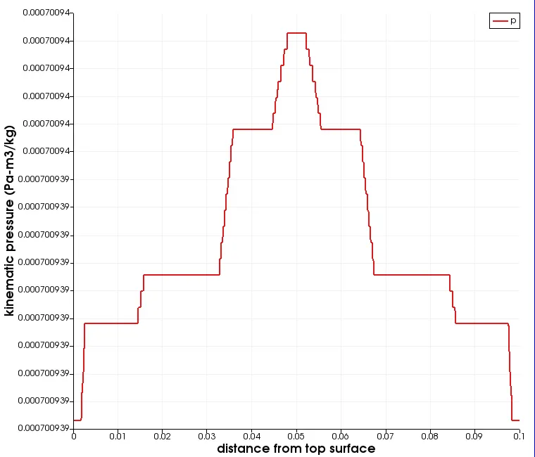
FIG - At t = 300sec, L = 5m from inlet
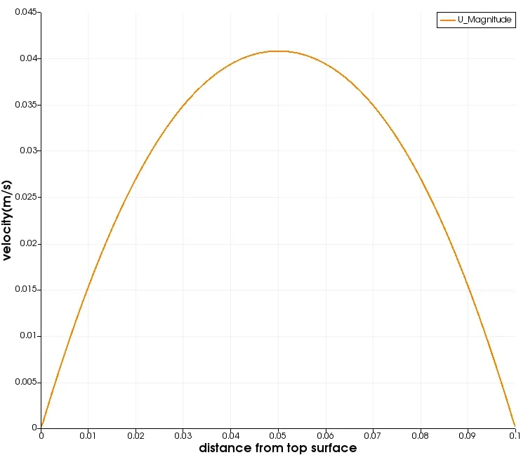
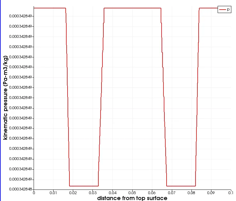
FIG - At t = 300sec, L = 10m from inlet
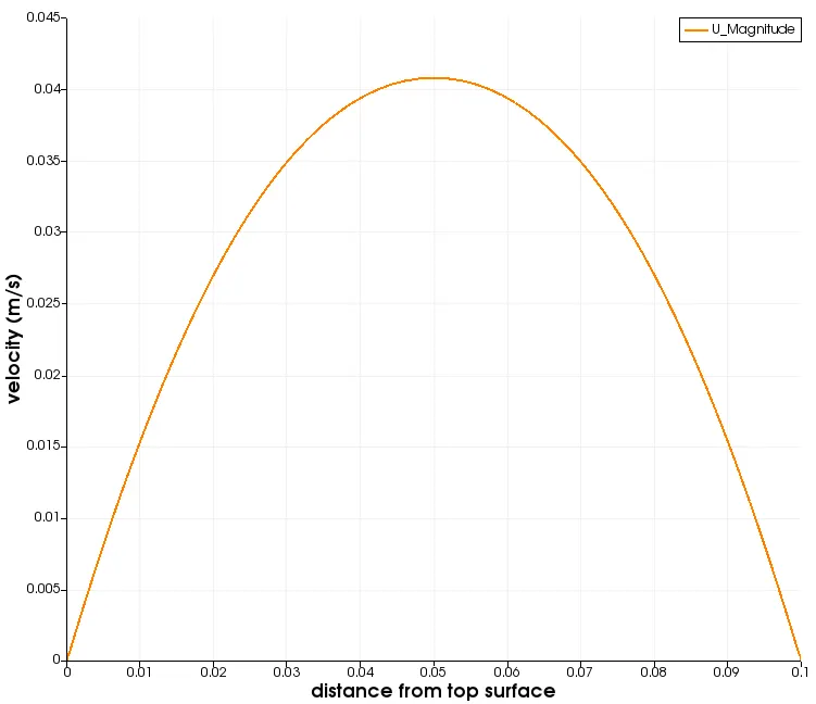
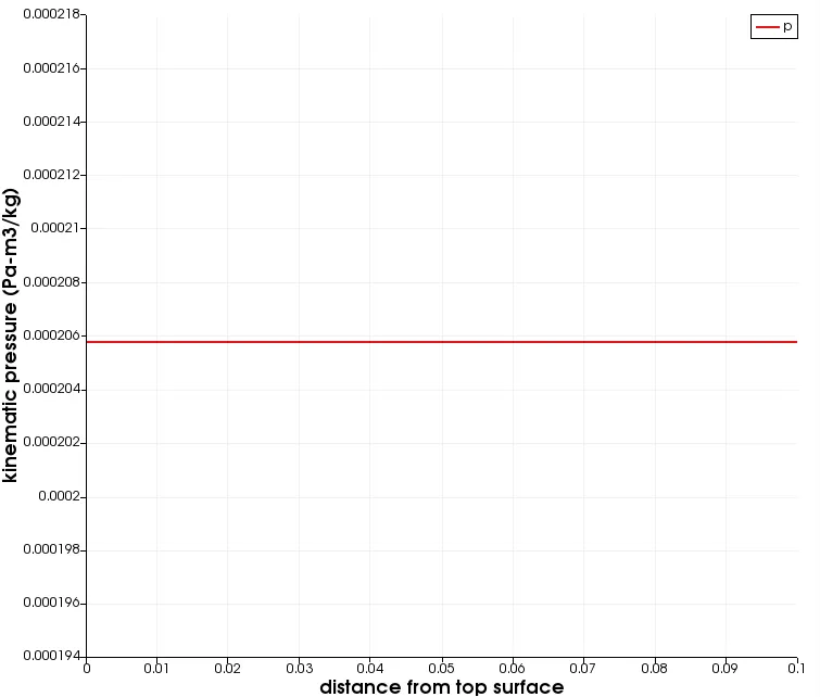
FIG - At t = 300sec, L = 12m from inlet
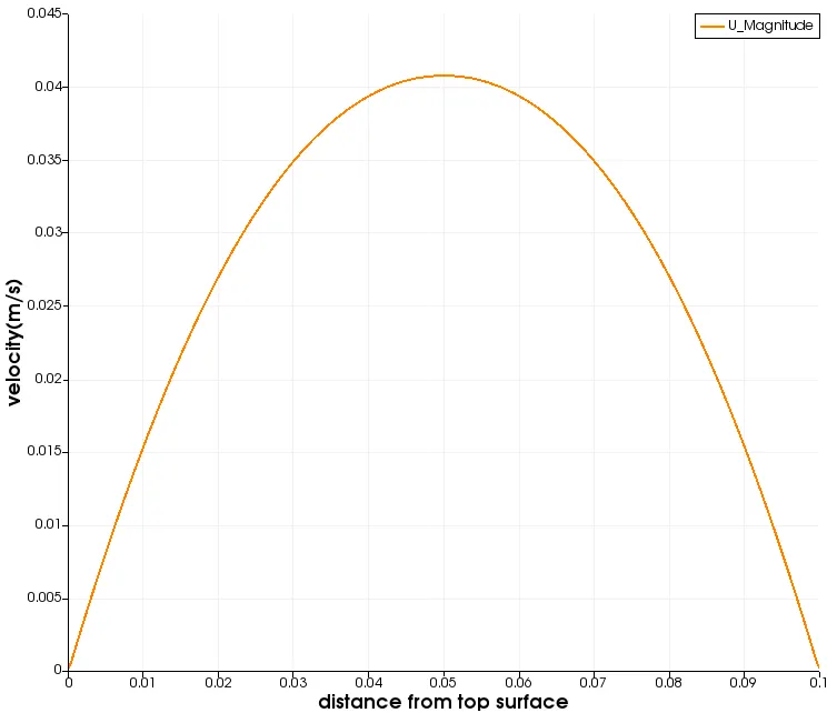
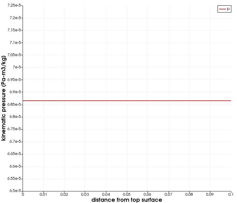
FIG - At t = 300sec, L = 14m from inlet
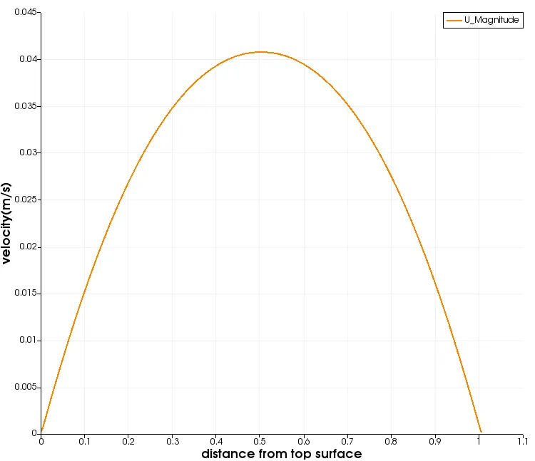
FIG - At t = 300sec, L = 15 m from inlet
Since, the pressure gradient is zero from L =12m, it is assumed that flow becomes fully developed after L = 12m from inlet of the pipe. The max velocity = 0.041 m/s.
Pressure plot -
NOTE - Hagen-poiseuille equations are derived only for fully developed region.
In Hagen-poiseuille equation describes the pressure drop due to viscosity of the fluid. So inorder to have a flow through out the pipe, pressure difference must exist. So Poiseuille equation provides the pressure gradient that must be provided between inlet and outlet for the fluid to flow.
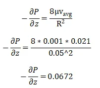
Since, Kinematic pressure is used in openFoam, -dp/dz = 0.0000672 (Pa-m2/kg)
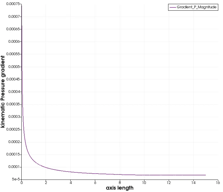
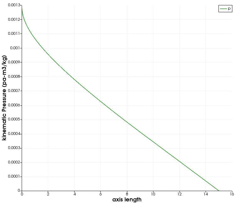
From the plot, inlet kinematic gauge pressure is 0.00127423 (Pa-m3/kg) and outlet gauge pressure is zero.
Shear-stress plot -
Since only velocity and pressure inlet conditions are given in openFoam, so only velocity and kinematic pressure fields are calculated. So, inorder to calculate other field variables, we have to follow certain steps.
Given, Shear stress = mu*du/dy
Step 1 - Calculate magnitude of absolute velocity
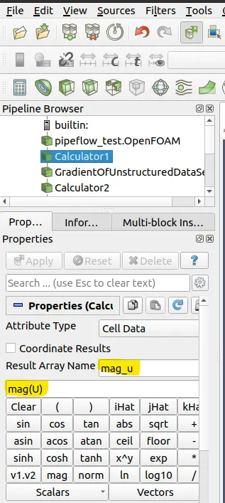
Step 2 - Calculate the gradient of velocity by FILTERS > SEARCH > GRADIENT OF UNSTRUCTURED DATA SET
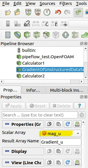
Step 3 - input the shear stress formula in the calculator
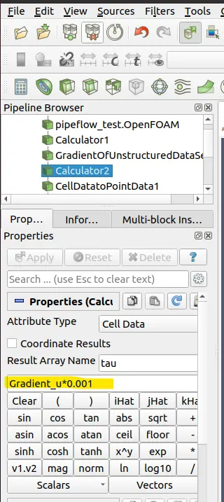
Step 4 - Plot the data
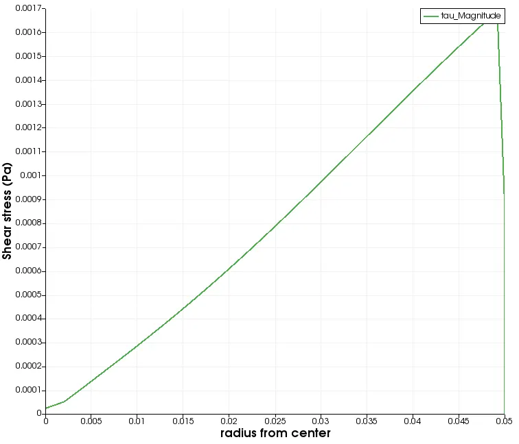
From the fig, the shear stress is maximum at the wall and is of magnitude 0.0017Pa and at the center of pipe it is almost zero. Since, magnitude is considered, the sign convention is neglected.
ANALYTICAL SOLUTIONS -
The results are plotted in matlab
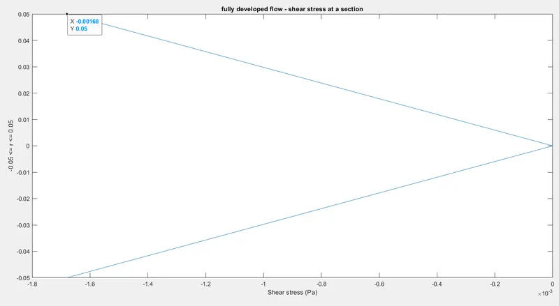
1)Shear stress
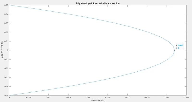
2)Velocity profile
| S.No | Field variable | magnitude of Analytical solution | magnitude of Numerical solution(OpenFoam) |
| 1 | Wall shear stress | 0.00168 Pa | 0.0017 Pa |
| 2 | Max velocity | 0.042 m/s | 0.041 m/s |
CONCLUSION:
The Hagen-poiseuille flow is simulated in openFoam and it shows accurate results. The steady state is reached after 300sec.