Week 11 - Simulation of Flow through a pipe in OpenFoam
Simulation of axisymmetric flow using OpenFOAM
Objective:
The aim of this project is to simulate the flow of water through a pipe and validate the results of the fully developed flow with analytical solutions.
Introduction:
The internal flow through the pipe is an axisymmetric problem. Hence the simulation is simplified to a wedge geometry as shown in the figure
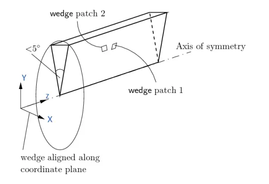
The wedge angle should be limited to a value of 5° to negate the effect of wall curvature. If the angle exceeds the limit of 5°, then the wall curvature should also be taken into account in the simulation. Therefore, here a wedge angle of 5° was used.
Since the objective of this study is to validate the fully-developed flow simulation, the length of the pipe should be chosen so that it is greater than the hydrodynamic entry length.
Hydrodynamic length is the length the fluid must travel inside a pipe before it becomes fully developed. Normally, the fluid would enter the pipe with uniform velocity. As the surface of the pipe is stationary, the layer of the fluid coming in contact with the pipe surface also becomes stationary due to the no-slip condition. The viscous forces within the fluid resist the adjacent layers leading to the development of a velocity profile with high velocity at the centre of the pipe [1]. This phenomenon is illustrated in the figure below:
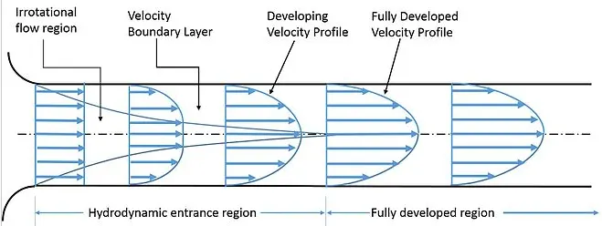
The entrance length depends on the velocity of the fluid, its density and viscosity. For a laminar flow, it can be calculated using the following equation [1]:
`L_(h,laminar) = 0.05*Re_D*D`
Where `Re_D = (rho*v*D)/(mu)` is the Reynolds number of the fluid.
`D` - diameter of the pipe
`rho` - density of fluid
`mu ` dynamic viscosity of the fluid
`v` - velocity of the fluid
In this project, water (`rho = 1000 (kg)/(m^3)` , `mu = 10^(-3)`) is the working fluid.
Hence, entrance length turns out to be `L_(h,laminar) = 0.05*2100*0.1 = 10.5 m`
In this project, the laminar flow with a Reynolds number of 2100 is simulated. With a little manipulation, the velocity of the fluid at the pipe entrance was calculated as `0.021 m/s`
Summary of the Domain setup
|
Parameter |
Value |
|
Diameter of pipe |
`0.1 m` |
|
Length of pipe |
`12 m` |
|
Wedge angle |
`5 deg` |
|
Working fluid |
Water @ `20°C` |
|
Density |
1000 `Kg/m^3` |
|
Dynamic viscosity |
`1*10^-3` `Pa-s` |
Mesh Setup:
The “Block Mesh” utility of OpenFOAM was used to generate the mesh. To generate a wedge geometry, the two vertices at the circumference of the wedge should be symmetrical [2]. A Matlab script was used to generate the blockMeshDict file used in the simulation and it is attached in the appendix. It generates the file based on the inputs supplied and it then can be used with OpenFOAM.
In order to simulate a 2D case, the number of cells along the x-direction was set to 1. Here the pipe extends in the z-direction.
Summary of the simulation setup:
|
Parameter |
Value |
|
Number of cells along z |
`200` |
|
Number of cells along y |
`20` |
|
Time step size |
`0.05 s` |
|
End time |
`550 s` |
Results and Discussion:
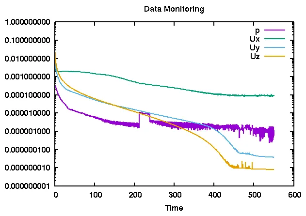
Since the flow is laminar and incompressible, the icoFOAM solver was chosen in this project. The simulation was carried till an end time of 550 s to allow the flow to become fully developed. The residuals object was added to monitor the residuals on the go. The evolution of the residuals is shown below.
The following figure shows the contour plot of velocity along the pipe in the entry region and the
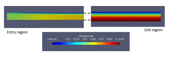
In the entry region, because of the no-slip boundary condition, the development of the boundary layer can be visualized. The velocity gradients in the radial direction changes along the pipe. On the other hand, in the exit region, the fully developed flow can be visualized with the constant velocity profile (radial velocity gradient).
Pressure drop:
From the simulation, the pressure was plotted along the axial direction
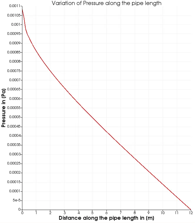
It can be observed that pressure drop decreases along the axial direction. In a horizontal pipe with a constant diameter, the pressure drop is the only force that is driving the flow. From the figure, the pressure drop was determined to be 1.1 Pa. Hagen Poiseuille equation can be used to validate the pressure drop obtained from the simulation [3].
According to the Hagen-Poiseuille equation, the pressure drop in a laminar incompressible flow through a cylindrical pipe with constant cross-section is given by
`Deltap=(8*mu*L*Q)/(pi*R^4)`
Where
`Deltap` - pressure drop in the cylindrical pipe in Pa
`mu` - dynamic viscosity in `Pa*s`
`L` - length of the pipe in `m`
`Q` - volumetric flow rate in `(m^3)/s`
`R` - radius of the pipe in `m`
Using this equation, the pressure is calculated as
`Deltap = (8*10^-3*12*pi*0.05^2*0.021)/(pi*0.05^4) = 0.8064 Pa`
Radial velocity:
In order to quantitatively visualise this development of the flow, the radial velocity profile was plotted at different axial distance (z-distance) as shown in the figure below
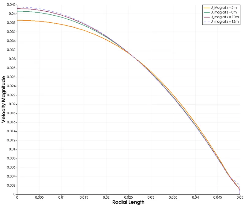
It can be observed that the distance of the velocity profile changes with increasing z-distance and it becomes constant after 10.5 m which is the same as obtained in the previous section. At the exit of the pipe, maximum velocity was found to be `0.04149 m/s` at the centre of the pipe.
The analytical velocity profile for a fully developed flow can be obtained from the formula [4]
`u(r) = V_c*(1-(r^2)/(R^2))`
Where
`V_c = (Deltap*D^2)/(16*mu*l)` - is the centreline velocity in [m/s]
`R` - is the pipe radius in [m]
`u(r)` is the velocity along the radial direction in [m/s]
From the above formula,
`V_c = (0.8064*0.1^2)/(16*10^(-3)*12) = 0.042 m/s`
In comparison with the analytical solution above, it can be observed that the value from the simulation is close to the analytical value with a error of 1.2%
Using the above formula for the velocity profile, the velocity at the exit of the pipe was calculated and plotted with the one obtained from simulation as shown in the following figure
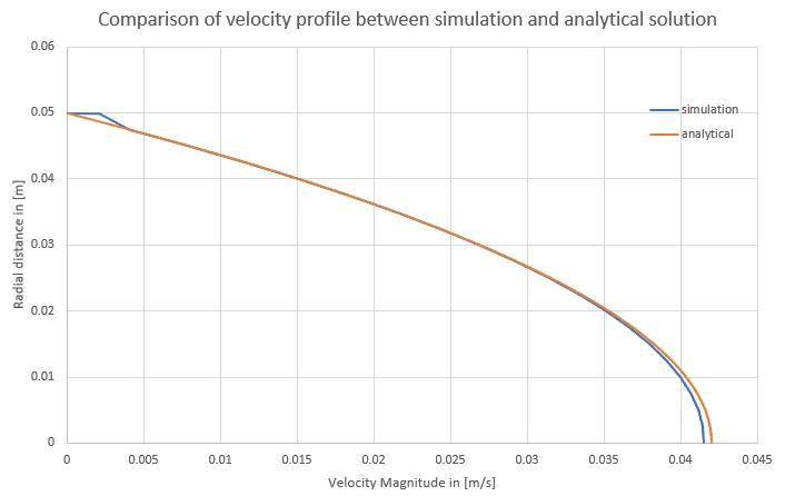
From the above figure, it can be observed that the velocity profile from the simulation is close to the analytical solution.
Wall Shear Stress:
In fluids, the wall shear stress is given by
`tau_w = mu*(du/dy)`
From the simulation results, first, the velocity gradient was determined using the “Gradient of Unstructured Data Set” option in Paraview. Then the dynamic viscosity is multiplied with the gradient to calculate the wall shear stress.
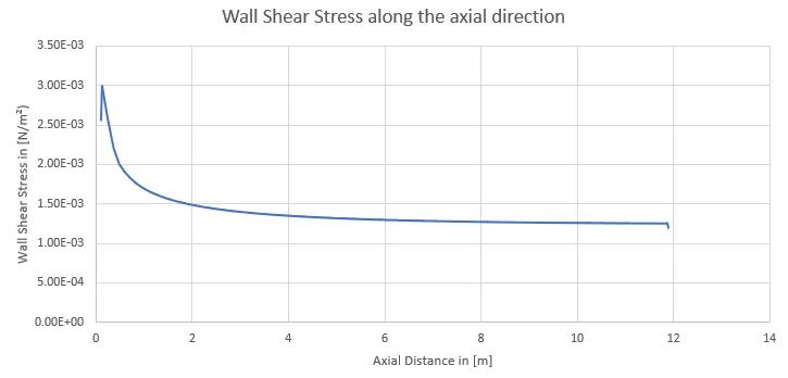
From the above figure, it can be seen that the wall shear stress is high at the pipe entrance and it decreases along the pipe. This is because at the entrance the velocity gradient is high and once the flow is fully developed, the velocity gradient becomes constant and hence the wall shear stress. The wall shear stress at the exit was found to be `1.19*10^(-3) N/(m^2)`
Analytically, the wall shear stress can be found for a fully developed flow using the following formula
`tau_w = (Deltap*D)/(4*L) = (0.8064*0.1)/(4*12) = 1.68*10^(-3)`
In comparison, the simulation result is slightly lower than the exact value.
Conclusion:
In this project, the axisymmetric internal flow through the pipe was simulated using wedge geometry and the results obtained from the simulation were validated using analytical results.
Here the transient case was solved and the simulation was performed for 550s which is more than enough time for the flow to transverse through the pipe of length 12m with an initial velocity of 0.021 m/s. If the simulation was performed for less than this value, then the results obtained would be far from the analytical value although the residual seems to be converged.
References:
- Entrance length (fluid dynamics) - Wikipedia
- Main ContribExamples/AxiSymmetric - OpenFOAMWiki^
- Hagen–Poiseuille equation - Wikipedia
- WEEK 12 OF AQS110 FLUID MECHANICS.pdf (ankara.edu.tr)
Appendix:
%% script to generate the blockMeshDict file
clear all
close all
clc

%% inputs
filename="blockMeshDict";

length = 12; %m
wedgeAngle = 5; %deg
dia = 0.1; % m
convertToMeters=1; % [-]

x_dis = (dia/2)*sind(wedgeAngle/2);
y_dis = (dia/2)*cosd(wedgeAngle/2);

% Vertices
v(1).name = '0';
v(1).coord = [0 0 0];

v(2).name = '1';
v(2).coord = [x_dis,y_dis,0];

v(3).name = '2';
v(3).coord = [-x_dis,y_dis,0];

v(4).name = '3';
v(4).coord = [0 0 length];

v(5).name = '4';
v(5).coord = [x_dis,y_dis,length];

v(6).name = '5';
v(6).coord = [-x_dis,y_dis,length];

% blocks
blocks(1).type = 'hex';
blocks(1).value = [0 0 1 2 3 3 4 5];
blocks(1).numCells = [1 20 100];
blocks(1).gradingType = 'simpleGrading';
blocks(1).gradingValue = [1 1 1];

% boundary faces
bc(1).name = 'inlet';
bc(1).type = 'patch';
bc(1).faces = [0 0 2 1];

bc(2).name = 'outlet';
bc(2).type = 'patch';
bc(2).faces = [3 4 5 3];

bc(3).name = 'outerWall';
bc(3).type = 'wall';
bc(3).faces = [2 5 4 1];

bc(4).name = 'front';
bc(4).type = 'wedge';
bc(4).faces = [5 2 0 3];

bc(5).name = 'back';
bc(5).type = 'wedge';
bc(5).faces = [0 1 4 3];

bc(6).name = 'axis';
bc(6).type = 'empty';
bc(6).faces = [3 3 0 0];

%%


fileId = fopen(filename,'w');
% file header
fprintf(fileId,'%s\n','/*--------------------------------*- C++ -*----------------------------------*\');
fprintf(fileId,'%s\n','  =========                 |');
fprintf(fileId,'%s\n','  \\      /  F ield         | OpenFOAM: The Open Source CFD Toolbox');
fprintf(fileId,'%s\n','   \\    /   O peration     | Website:  https://openfoam.org');
fprintf(fileId,'%s\n','    \\  /    A nd           | Version:  6');
fprintf(fileId,'%s\n','     \\/     M anipulation  |');
fprintf(fileId,'%s\n',' \*---------------------------------------------------------------------------*/');
fprintf(fileId,'%s\n',' FoamFile');
fprintf(fileId,'%s\n',' {');
fprintf(fileId,'%s\n','     version     2.0;');
fprintf(fileId,'%s\n','     format      ascii;');
fprintf(fileId,'%s\n','     class       dictionary;');
fprintf(fileId,'%s\n','     object      blockMeshDict;');
fprintf(fileId,'%s\n',' }');
fprintf(fileId,'%s\n','// * * * * * * * * * * * * * * * * * * * * * * * * * * * * * * * * * * * * * //');
fprintf(fileId,'%s\n',' ');
fprintf(fileId,'%s\t%0.4f%s\n','convertToMeters',convertToMeters,';');
fprintf(fileId,'%s\n',' ');

for i=1:size(v,2)
    last=false;
    if i==size(v,2)
        last=true;
    end
    writeVertices(fileId,i,v(i),last);
end

for i=1:size(blocks,2)
    last=false;
    if i==size(blocks,2)
        last=true;
    end
    writeBlocks(fileId,i,blocks(i),last);
end

% edges
fprintf(fileId,'%s\n','edges');
fprintf(fileId,'%s\n','(');
fprintf(fileId,'%s\n',');');
fprintf(fileId,'%s\n',' ');

for i=1:size(bc,2)
    last=false;
    if i==size(bc,2)
        last=true;
    end
    writeBCs(fileId,i,bc(i),last);
end

% Merge Patches
fprintf(fileId,'%s\n','mergePatchPairs');
fprintf(fileId,'%s\n','(');
fprintf(fileId,'%s\n',');');
fclose(fileId);


%% functions
function writeVertices(fileId,num,v,last)
    if num == 1
        fprintf(fileId,'%s\n','vertices ');
        fprintf(fileId,'%s\n','(');
    end
    fprintf(fileId,'\t( %0.4f %0.4f %0.4f )\t%s%s\n',v.coord,'//',v.name);
    if last

        fprintf(fileId,'%s\n',');');
        fprintf(fileId,'%s\n',' ');

    end

end

function writeBlocks(fileId,num,block,last)

    if num == 1
        fprintf(fileId,'%s\n','blocks ');
        fprintf(fileId,'%s\n','(');
    end
    fprintf(fileId,'\t%s (%d %d %d %d %d %d %d %d) (%d %d %d) %s (%d %d %d)\n',block.type,block.value,block.numCells,block.gradingType,block.gradingValue);
    if last

        fprintf(fileId,'%s\n',');');
        fprintf(fileId,'%s\n',' ');

    end

end

function writeBCs(fileId,num,bc,last)
    if num == 1
        fprintf(fileId,'%s\n','boundary ');
        fprintf(fileId,'%s\n','(');
    end
    fprintf(fileId,'\t%s\n',bc.name);
    fprintf(fileId,'\t%s\n','{');
    fprintf(fileId,'\t\t%s\t%s%s\n','type',bc.type,';');
    fprintf(fileId,'\t\t%s\n','faces');
    fprintf(fileId,'\t\t%s\n','(');
    fprintf(fileId,'\t\t\t(%d %d %d %d)\n',bc.faces);
    fprintf(fileId,'\t\t%s\n',');');
    fprintf(fileId,'\t%s\n','}');
    if last

        fprintf(fileId,'%s\n',');');
        fprintf(fileId,'%s\n',' ');

    end

end