Week 11 - Simulation of Flow through a pipe in OpenFoam
1. Title – Simulation of Flow through Pipe OpenFoam.
2. Objective –
- To automate blockmeshdict file using MATLAB which contains pipe dimension and boundaries.
- To setup the initial and boundary conditions for simulation and run with a suitable solver.
- Create pressure and velocity contours and profiles using paraview and validate them.
3. Introduction –
A common situation encountered by the CFD engineer is fluid flow through a tube or pipe. This occurs in heat exchangers, water management systems, oil transport in refineries etc. so it becomes important to know about the losses, pressure drop, velocity of fluid and these determines the efficiency of pipe to flow the fluid. In this study we are going simulate laminar-incompressible fluid flow through a pipe. We will generate velocity profile and identify the hydrodynamic length and fully developed flow.
4. Theory –
Flows completely bounded by solid surfaces are called internal flows, which include flows through pipes, nozzles, diffusers, valves, and fittings. The basic principles involved are independent of the cross-sectional shape, although the details of the flow may be dependent on it. The flow regime which is laminar or turbulent, of internal flows is primarily depends a function of Reynolds number. Laminar flow can be solved analytically, on the basis of that we assumed laminar flow for this study and we will draw some results analytically and then we will validate simulation results with analytical results.
In fluid dynamics, the Hagen–Poiseuille equation, also known as the Hagen–Poiseuille law, is a physical law that gives the pressure drop in a fluid flowing through a long cylindrical pipe. The assumptions of the equation are that the fluid is incompressible and Newtonian; the flow is laminar through a pipe of constant circular cross-section that is substantially longer than its diameter; and there is no acceleration of fluid in the pipe.
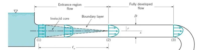
Any fluid flowing in a pipe had to enter the pipe at some location. The region of flow near where the fluid enters the pipe is termed the entrance region or developing region. As the fluid moves through the pipe, viscous effects cause it to stick to the pipe wall. Initial velocity profile changes with distance along the pipe x, until the fluid reaches the end of the entrance length, beyond which the velocity profile does not vary with x.
Pressure Distribution along the pipe –
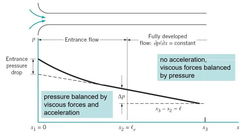
In the entrance region of a pipe, the fluid accelerates or decelerates as it flows. there is a balance between pressure, viscous and inertia force and in fully developed pressure gradient is constant.
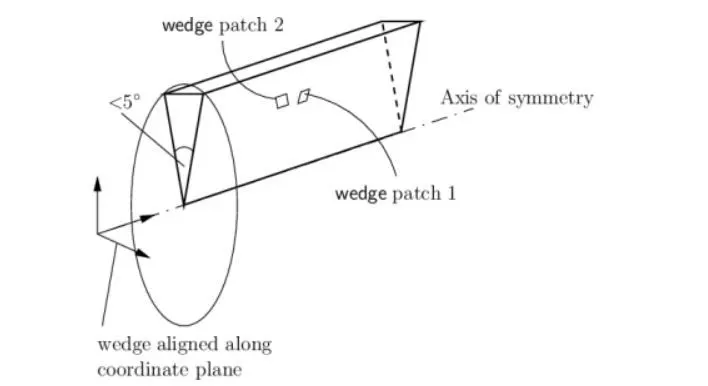
Wedge Boundary conditions - For two dimensional axi-symmetric cases, like a cylinder, the geometry is specified as a wedge of small angle less than 5degree and 1 cell thick running along the plane of symmetry, as shown in Figure, above. The axi-symmetric wedge planes must be specified as separate patches of wedge type.
Understanding the geometry or blockMeshdict file –
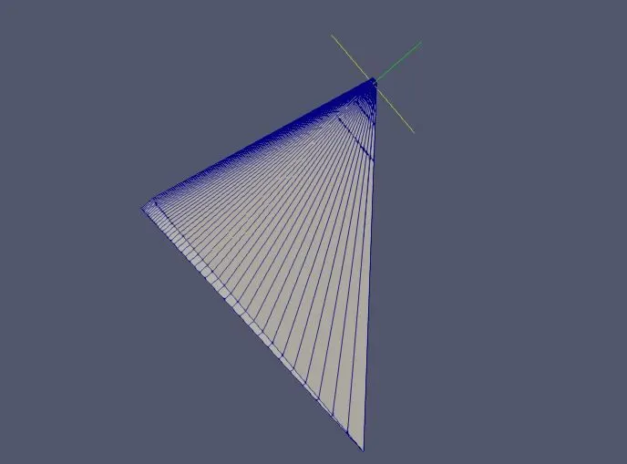
The following image is the sector of pipe-
We can see there are six vertices, in vertices section of blockMeshDict file we need to define them. There are two arcs which will be defined by length of pipe and pipe diameter, in the edges section of the blockmesh File.
Vertices … (0 0 0), (0 y z) … here y and z are the distance of particular vertex from origin.
Edges…arc vertices number (0 d 0) and arc vertices number (L d 0)
For meshing define the type of mesh then vertices number then number of cell in all three direction followed by grading factor.
hex (0 3 5 2 0 3 4 1) (80 40 1) simpleGrading (0.01 0.05 0.1)
In boundary condition we need to define the inlet, outlet and wall patches so for inlet and outlet we can write
Inlet (0 1 2 0)
Similarly other boundaries can be defined.
Pipe and fluid parameters –
Type of fluid – water
Density of fluid = `997(kg)/m^3`
Reynold number = 2100
Dynamic viscosity(mho) = `8.90*10^-4 Pa*s`
Length of pipe(L) = 4m
Diameter of pipe(d) = 0.025m
Wedge angle = 2.5
Formulas and calculations –
1. Entry length = `0.06*R_e*D`= `0.06*2100*0.025` =`3.15m`
2. Average velocity = `R_e*(mho)/(rho*d)`= `(2100*8.90*10^-4)/(997*0.025)` = `0.0749m/s`
3. Maximum velocity = 2*average velocity = `2*0.0749` = `0.1498 m/s`
4. Pressure difference = `(32*mho*L*v_(avg))/(d^2)` = `(32*8.90*10^-4*4*0.0749)/(0.025)^-2` = `13.65Pa`
5. Kinematic pressure drop = pressure difference/rho = `13.65/997`= `0.01369 (m/s)^2`
5. Procedure –
We are simulating flow through pipe, for that we wrote a programme in MATLAB which replicates the blockMeshdict file. In MATLAB this file saved as text file and text file is directly copied into existing blockMeshDict file. The process has automated because it generates blockMeshdict file automatically after asking the length of pipe, diameter of pipe and wedge angle.
MATLAB code -
clear all
close all
clc

% pipe dimensions and fluid parameter
Re = 2100;
mho = 8.90*10^-4;
rho = 997;
nu = 8.917*10^-7;
% user inputs
% diameter of pipe
d = input('Enter pipe diameter - ');
% length of pipe
L =   input('Enter the length of pipe - ');
% wedge angle of pipe
w_a = input('Enter the wedge angle of pipe - ');

% entry length
L_e = 0.06*Re*d;
% average velocity
v_avg = Re*nu/d;
% pressure drop
P_drop = 32*mho*v_avg*L/(d^2);

% these parameter will be used to calculate vertices along y and z axis
y = (d/2)*cosd(w_a/2);
z = (d/2)*sind(w_a/2);

% opening text file
b_m = fopen('blockMeshDict.txt','w');

% writing first few lines
l = 'FoamFile';
l1 = '{';
l2 = 'version    2.0;';
l3 = 'format     ascii;';
l4 = 'class      dictionary;';
l5 = 'object     blockMeshDict;';
l6 = '}';
l7 = 'convertToMeters 1;';
fprintf(b_m,'%s\n%s\n%s\n%s\n%s\n%s\n%s\n',l,l1,l2,l3,l4,l5,l6,l7);


% printing vertices
fprintf(b_m,'\nvertices\n');
fprintf(b_m,'(\n');
fprintf(b_m,'(0 0 0)\n');
fprintf(b_m,'(0 %s %s)\n',y,z);
fprintf(b_m,'(0 %s -%s)\n',y,z);
fprintf(b_m,'(%f 0 0)\n',L);
fprintf(b_m,'(%f %s %s)\n',L,y,z);
fprintf(b_m,'(%f %s -%s)\n);\n\n',L,y,z);
% meshing data
fprintf(b_m,'blocks\n');
fprintf(b_m,'(\n hex (0 3 5 2 0 3 4 1) (80 40 1) simpleGrading (0.01 0.05 0.1)\n);\n\n');
% edges
fprintf(b_m,'edges\n(\n arc 1 2 (0 %f 0)\n',d/2);
fprintf(b_m,' arc 4 5 (%f %f 0)\n);\n\n',L,d/2);
% defining boundaries
fprintf(b_m,'boundary\n(\n');
fprintf(b_m,'axis\n{\n');
fprintf(b_m,' type  empty;\n faces\n(',d/2);
fprintf(b_m,'(0 3 3 0));\n}\n',L,d/2);

fprintf(b_m,'wall\n{\n');
fprintf(b_m,' type  wall;\n faces\n(',d/2);
fprintf(b_m,'(1 4 5 2));\n}\n',L,d/2);

fprintf(b_m,'inlet\n{\n');
fprintf(b_m,' type  patch;\n faces\n(',d/2);
fprintf(b_m,'(0 1 2 0));\n}\n',L,d/2);

fprintf(b_m,'outlet\n{\n');
fprintf(b_m,' type  patch;\n faces\n(',d/2);
fprintf(b_m,'(3 5 4 3));\n}\n',L,d/2);

fprintf(b_m,'front\n{\n');
fprintf(b_m,' type  wedge;\n faces\n(',d/2);
fprintf(b_m,'(0 3 4 1));\n}\n',L,d/2);

fprintf(b_m,'back\n{\n');
fprintf(b_m,' type  wedge;\n faces\n(',d/2);
fprintf(b_m,'(0 2 5 3));\n}\n);\n\n',L,d/2);

fprintf(b_m,'mergePatchPairs\n();');
% closing text file
fclose(b_m);
After text file generated from MATLAB, we copied data to blockMeshdict file and ran blockMeshdict.exe and paraFoam command in terminal to preview the model of pipe.
blockMeshDict file -
FoamFile
{
version    2.0;
format     ascii;
class      dictionary;
object     blockMeshDict;
}
convertToMeters 1;

vertices
(
(0 0 0)
(0 1.249703e-02 2.726861e-04)
(0 1.249703e-02 -2.726861e-04)
(4.000000 0 0)
(4.000000 1.249703e-02 2.726861e-04)
(4.000000 1.249703e-02 -2.726861e-04)
);

blocks
(
 hex (0 3 5 2 0 3 4 1) (80 40 1) simpleGrading (0.01 0.05 0.1)
);

edges
(
 arc 1 2 (0 0.012500 0)
 arc 4 5 (4.000000 0.012500 0)
);

boundary
(
axis
{
 type  empty;
 faces
((0 3 3 0));
}
wall
{
 type  wall;
 faces
((1 4 5 2));
}
inlet
{
 type  patch;
 faces
((0 1 2 0));
}
outlet
{
 type  patch;
 faces
((3 5 4 3));
}
front
{
 type  wedge;
 faces
((0 3 4 1));
}
back
{
 type  wedge;
 faces
((0 2 5 3));
}
);

mergePatchPairs
();
Initial and Boundary conditions -
Pressure -
/*--------------------------------*- C++ -*----------------------------------*\
| =========                 |                                                 |
| \\      /  F ield         | OpenFOAM: The Open Source CFD Toolbox           |
|  \\    /   O peration     | Version:  v2012                                 |
|   \\  /    A nd           | Website:  www.openfoam.com                      |
|    \\/     M anipulation  |                                                 |
\*---------------------------------------------------------------------------*/
FoamFile
{
    version     2.0;
    format      ascii;
    class       volScalarField;
    object      p;
}
// * * * * * * * * * * * * * * * * * * * * * * * * * * * * * * * * * * * * * //

dimensions      [0 2 -2 0 0 0 0];

internalField   uniform 0;

boundaryField
{
    axis
    {
        type            empty;
    }

    wall
    {
        type            zeroGradient;
    }

   inlet
    {
        type            zeroGradient;
    }

    outlet
    {
        type            fixedValue;
        value           uniform 0.017116;
    }
    front
    {
        type            wedge;
    }
    back
    {
        type            wedge;
    }
}******************************************************************** //
Velocity -
/*--------------------------------*- C++ -*----------------------------------*\
| =========                 |                                                 |
| \\      /  F ield         | OpenFOAM: The Open Source CFD Toolbox           |
|  \\    /   O peration     | Version:  v2012                                 |
|   \\  /    A nd           | Website:  www.openfoam.com                      |
|    \\/     M anipulation  |                                                 |
\*---------------------------------------------------------------------------*/
FoamFile
{
    version     2.0;
    format      ascii;
    class       volVectorField;
    object      U;
}
// * * * * * * * * * * * * * * * * * * * * * * * * * * * * * * * * * * * * * //

dimensions      [0 1 -1 0 0 0 0];

internalField   uniform (0.0749 0 0);

boundaryField
{
    axis
    {
        type            empty;
    }

    wall
    {
        type            noSlip;
    }

   inlet
    {
        type            fixedValue;
        value           uniform (0.0749 0 0);
    }

    outlet
    {
        type            zeroGradient;
    }
    front
    {
        type            wedge;
    }
    back
    {
        type            wedge;
    }
}

// ************************************************************************* //
Physical Properties -
/*--------------------------------*- C++ -*----------------------------------*\
| =========                 |                                                 |
| \\      /  F ield         | OpenFOAM: The Open Source CFD Toolbox           |
|  \\    /   O peration     | Version:  v2012                                 |
|   \\  /    A nd           | Website:  www.openfoam.com                      |
|    \\/     M anipulation  |                                                 |
\*---------------------------------------------------------------------------*/
FoamFile
{
    version     2.0;
    format      ascii;
    class       dictionary;
    location    "constant";
    object      transportProperties;
}
// * * * * * * * * * * * * * * * * * * * * * * * * * * * * * * * * * * * * * //

nu              [0 2 -1 0 0 0 0] 8.917e-7;


// ************************************************************************* //
Control file-
/*--------------------------------*- C++ -*----------------------------------*\
| =========                 |                                                 |
| \\      /  F ield         | OpenFOAM: The Open Source CFD Toolbox           |
|  \\    /   O peration     | Version:  v2012                                 |
|   \\  /    A nd           | Website:  www.openfoam.com                      |
|    \\/     M anipulation  |                                                 |
\*---------------------------------------------------------------------------*/
FoamFile
{
    version     2.0;
    format      ascii;
    class       dictionary;
    location    "system";
    object      controlDict;
}
// * * * * * * * * * * * * * * * * * * * * * * * * * * * * * * * * * * * * * //

application     pimpleFoam;

startFrom       startTime;

startTime       0;

stopAt          endTime;

endTime         20;

deltaT          0.01;

writeControl    timeStep;

writeInterval   20;

purgeWrite      0;

writeFormat     ascii;

writePrecision  6;

writeCompression off;

timeFormat      general;

timePrecision   6;

runTimeModifiable true;


// ************************************************************************* //
Solution and scheme -
fvSolution -
/*--------------------------------*- C++ -*----------------------------------*\
| =========                 |                                                 |
| \\      /  F ield         | OpenFOAM: The Open Source CFD Toolbox           |
|  \\    /   O peration     | Version:  v2012                                 |
|   \\  /    A nd           | Website:  www.openfoam.com                      |
|    \\/     M anipulation  |                                                 |
\*---------------------------------------------------------------------------*/
FoamFile
{
    version     2.0;
    format      ascii;
    class       dictionary;
    location    "system";
    object      fvSolution;
}
// * * * * * * * * * * * * * * * * * * * * * * * * * * * * * * * * * * * * * //

solvers
{
    p
    {
        solver          PCG;
        preconditioner  DIC;
        tolerance       1e-06;
        relTol          0.05;
    }

    pFinal
    {
        $p;
        relTol          0;
    }

    U
    {
        solver          smoothSolver;
        smoother        symGaussSeidel;
        tolerance       1e-05;
        relTol          0;
    }
}

PISO
{
    nCorrectors     2;
    nNonOrthogonalCorrectors 0;
    pRefCell        0;
    pRefValue       0;
}


// ************************************************************************* //
fvScheme -
/*--------------------------------*- C++ -*----------------------------------*\
| =========                 |                                                 |
| \\      /  F ield         | OpenFOAM: The Open Source CFD Toolbox           |
|  \\    /   O peration     | Version:  v2012                                 |
|   \\  /    A nd           | Website:  www.openfoam.com                      |
|    \\/     M anipulation  |                                                 |
\*---------------------------------------------------------------------------*/
FoamFile
{
    version     2.0;
    format      ascii;
    class       dictionary;
    location    "system";
    object      fvSchemes;
}
// * * * * * * * * * * * * * * * * * * * * * * * * * * * * * * * * * * * * * //

ddtSchemes
{
    default         Euler;
}

gradSchemes
{
    default         Gauss linear;
    grad(p)         Gauss linear;
}

divSchemes
{
    default         none;
    div(phi,U)      Gauss linear;
}

laplacianSchemes
{
    default         Gauss linear orthogonal;
}

interpolationSchemes
{
    default         linear;
}

snGradSchemes
{
    default         orthogonal;
}


// ************************************************************************* //
After writing for control parameters, boundary conditions we ran the command icoFoam.exe to solve the case and after paraFoam command executed again to generate desire result.
MATLAB Code used to generate velcoity profile -
clear all
close all
clc

% radius of the pipe
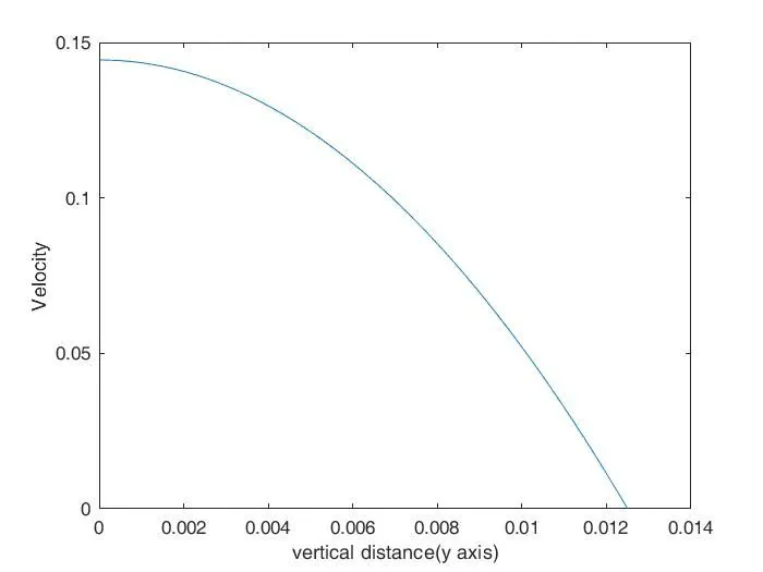
R = 0.0125;
% points along the radius
r = linspace(0,R,50);
% maximum velocity
v_max = 0.1444;

% velocity calculation along the radius
for i = 1:length(r)
v(i) = v_max*(1-(r(i)/R).^2);
end

% plotting
plot(r,v)
hold on
plot(-r,v)
xlabel('vertical distance(y axis)')
ylabel('Velocity')
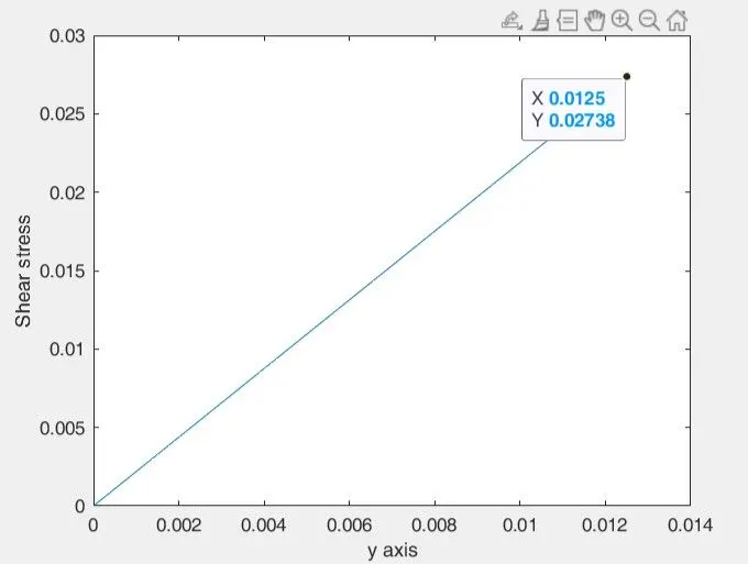
MATLAB Code used to calculate shear stress -
clear all
close all
clc

% dynamic viscosity
mho = 8.9*10^-4;
% maximum  velocity
v_max = 0.1498;
% pipe radius
R = 0.0125;
% points along the radius
r = linspace(0,R,100);
% pressure drop
dp = 0.01369;
% length of pipe
l = 4;

% shear stress calculation along the radius of pipe
for i = 1:length(r)
tau(i) = (dp/2*l)*(r(i)/R);
end

% plotting
plot(r,tau)
xlabel('y axis')
ylabel('Shear stress')
6. Results –
Geometry -
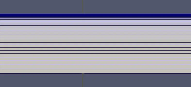
1. Hydrodynamic length analytical vs numerical – from analytical result we go hydrodynamic length 3.15m in calculation section, means after it, velocity profile will be fully developed. In simulation velocity graphs has created to identify the location of hydrodynamic length.
From the graph and table it is clear that velocity is not varing after 3.15m, along the diameter of pipe or y axis, so it validates analytical result.
Numerical results -
Velocity at 2m from inlet -
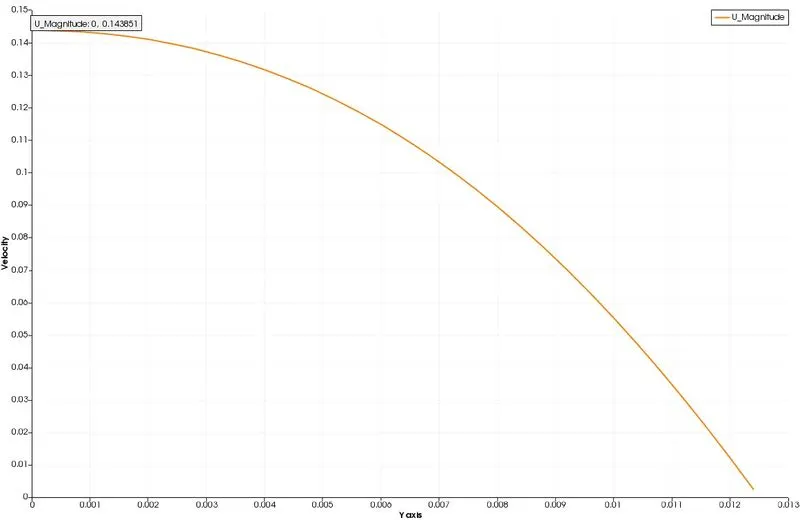
Velocity at 3.15m from inlet -
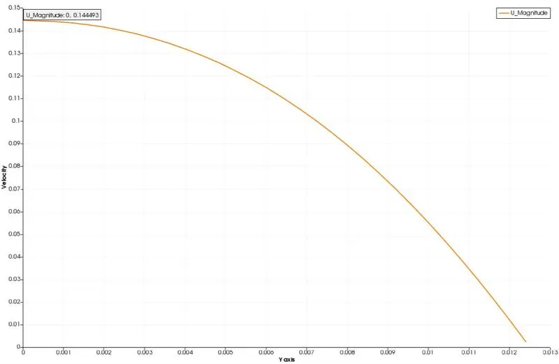
Velocity at 3.50m from inlet -
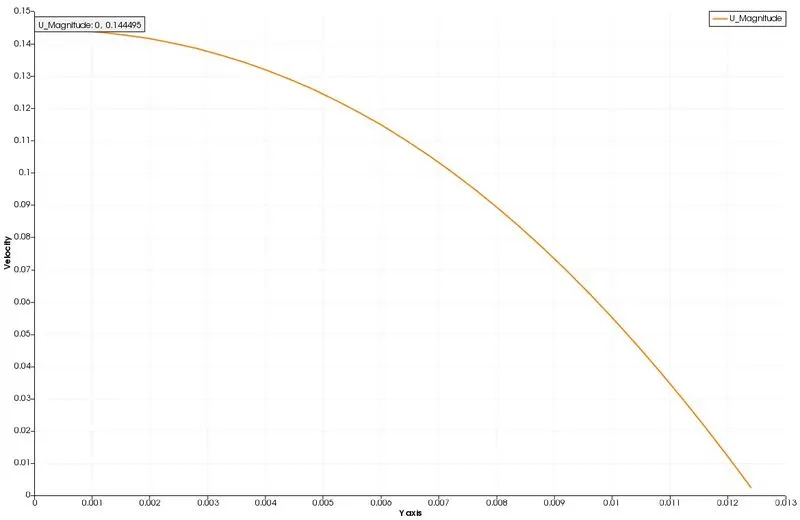
2. Fully flow developed profile analytic solution vs numerical solution
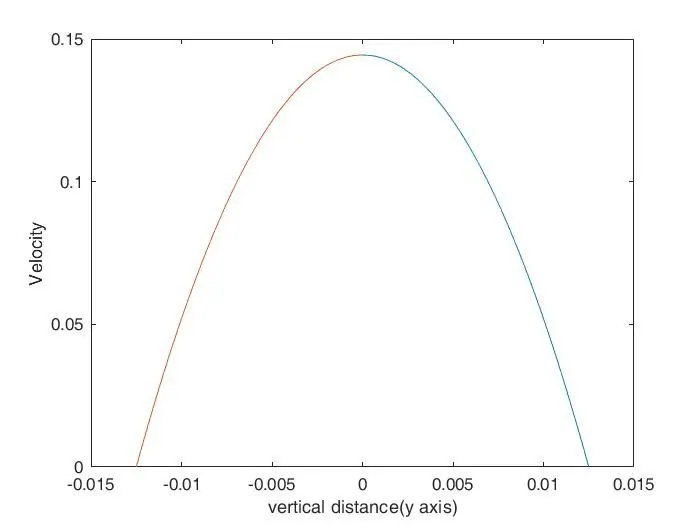
Form the graph it is easily seen that velocity profile is parabolic and it is matches with analytic solution. To plot velocity from the formula a separate MATLAB programme was written which is in the procedure.
Analytical -
Numerical -
3. Pressure drop and maximum velocity analytic solution vs numerical solution
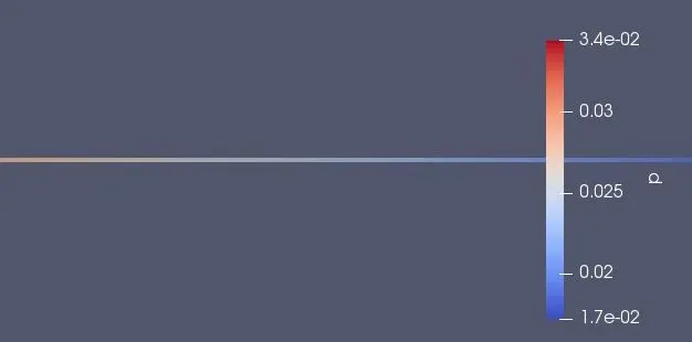
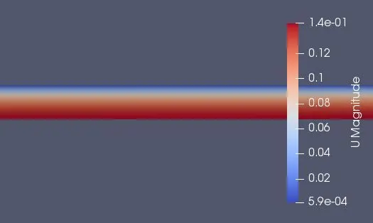
We got maximum velocity 0.1498m/s and from simulation we got 0.1444m/s, which is close to analytical one. the pressure drop from formula was 0.001369Pa and from contour we can calculate 0.0034 -0.0017 = 0.0017Pa.
Numerical -
Pressure contour -
Velocity contour -
4. Shear stress profile and wall shear stress analytic solution vs numerical solution –
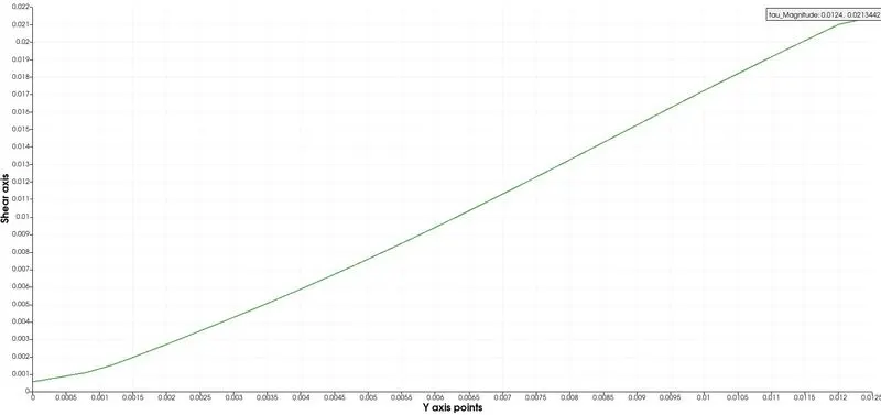
To calculate shear profile separate programme was written, from that we got wall shear stress 0.02738N/m^2 and we got 0.02134N/m^2 from simulation.
Analytic -
Numerical -
Results at a glance –
|
Variables/solution method |
Analytical |
Numerical |
|
Maximum velocity |
0.1498m/s |
0.1444m/s |
|
Kinematic Pressure drop |
0.01369Pa |
0.017Pa |
|
Wall shear stress |
0.02738N/m^2 |
0.02134N/m^2 |
|
Hydrodynamic length |
3.15 |
3.15 |