Simulation of Flow through a pipe in OpenFoam
Simulation of Laminar Flow through a Pipe in OpenFoam
Liquid or gas flow through pipes or ducts is commonly used in heating and cooling applications and fluid distribution networks. The fluid in such applications is usually forced to flow by a fan or pump through a flow section. The friction, which is directly related to the pressure drop and head loss during flow through pipes and ducts. The pressure drop is then used to determine the pumping power requirement. A typical piping system involves pipes of different diameters connected to each other by various fittings or elbows to route the fluid, valves to control the flow rate, and pumps to pressurize the fluid.
The fluid velocity in a pipe changes from zero at the wall because of the no-slip condition to a maximum at the pipe center. In fluid flow, it is convenient to work with an average velocity `V_(avg)`, which remains constant in incompressible flow when the cross-sectional area of the pipe is constant.
Laminar Flow
Laminar or streamline flow in pipes (or tubes) occurs when a fluid flows in parallel layers, with no disruption between the layers. At low velocities, the fluid tends to flow without lateral mixing, and adjacent layers slide past one another. There are no cross-currents perpendicular to the direction of flow, nor eddies or swirls of fluids. In laminar flow, the motion of the particles of the fluid is very orderly with all particles moving in straight lines parallel to the pipe walls. Any lateral mixing (mixing at right angles to the flow direction) occurs by the action of diffusion between layers of the liquid. Diffusion mixing can be slow however if the diameter of the pipe of the tube is small then this diffusive mixing can be very significant.
Turbulent Flow
Turbulent flow is a flow regime characterized by chaotic property changes. This includes a rapid variation of pressure and flows velocity in space and time. Turbulent flow is a type of fluid (gas or liquid) flow in which the fluid undergoes irregular fluctuations, or mixing, in contrast to laminar flow, in which the fluid moves in smooth paths or layers. In turbulent flow, the speed of the fluid at a point is continuously undergoing changes in both magnitude and direction.
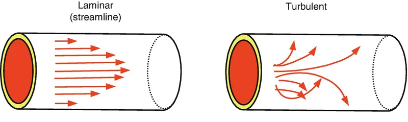
Most kinds of fluid flow are turbulent, except for laminar flow at the leading edge of solids moving relative to fluids or extremely close to solid surfaces, such as the inside wall of a pipe, or in cases of fluids of high viscosity (relatively great sluggishness) flowing slowly through small channels. Common examples of turbulent flow are blood flow in arteries, oil transport in pipelines, lava flow, atmosphere and ocean currents, the flow through pumps and turbines, and the flow in boat wakes and around aircraft-wing tips.
Reynolds Number
The Reynolds number is the ratio of inertial forces to viscous forces within a fluid that is subjected to relative internal movement due to different fluid velocities. A region where these forces change behaviour is known as a boundary layer, such as the bounding surface in the interior of a pipe.
The Reynolds number (`Re`) helps predict flow patterns in different fluid flow situations. At low Reynolds numbers, flows tend to be dominated by laminar (sheet-like) flow, while at high Reynolds numbers flows tend to be turbulent.
`Re=(rhoV_(avg)^2L^2)/(muV_(avg)L)=(rhoV_(avg)L)/(mu)=(V_(avg)L)/(nu)`
Reynolds Number for a internal flow through circular pipe is given as, `Re=(rhoV_(avg)D)/(mu)`
Reynolds number for flow through pipes
`Re<=2300` Laminar flow
`2300<=Re<=4000` Transitional flow
`Re>=4000` Turbulent Flow
Entrance Length
The entrance length is the distance a flow travels after entering a pipe before the flow becomes fully developed. Entrance length refers to the length of the entry region, the area following the pipe entrance where effects originating from the interior wall of the pipe propagate into the flow as an expanding boundary layer. When the boundary layer expands to fill the entire pipe, the developing flow becomes a fully developed flow, where flow characteristics no longer change with increased distance along the pipe. Many different entrance lengths exist to describe a variety of flow conditions.
The region from the pipe inlet to the point at which the velocity profile is fully developed is called the hydrodynamic entrance region, and the length of this region is called the hydrodynamic entry length `L_h`.
Velocity profile for Laminar flow
The hydrodynamic entry length is usually taken to be the distance from the pipe entrance to where the wall shear stress (and thus the friction factor) reaches within about 2% of the fully developed value.
For Laminar Flow
`L_(h,laminar)/D=0.05Re`
For `Re` 20, the hydrodynamic entry length is about the size of the diameter but increases linearly with velocity. In the limiting laminar case of `Re` 2300, the hydrodynamic entry length is 115D.
For Turbulent Flow
In turbulent flow, the intense mixing during random fluctuations usually overshadows the effects of molecular diffusion. The nondimensional hydrodynamic entry length for turbulent flow is approximated as
`L_(h,turbu l ent)/D=1.359Re^(1/4)`
The entrance effects become insignificant beyond a pipe length of about 10 diameters, and the nondimensional hydrodynamic entry length is approximated as
`L_(h,turbu l ent)/D=10`
Velocity Profile for Laminar Flow through Pipe
The velocity profile in a fully developed laminar flow in a pipe is parabolic with a maximum at the centerline and a minimum (zero) at the pipe wall. Also, the axial velocity `u` is positive for any `r`, and thus the axial pressure gradient `(dP)/dx` must be negative that is the pressure must decrease in the flow direction because of viscous effects—it takes pressure to push the fluid through the pipe.
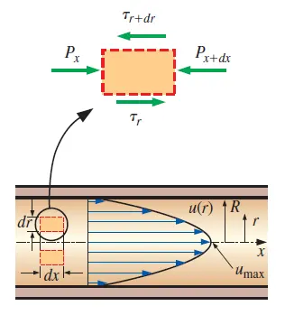
Velocity Profile
`u(r)=-R^2/(4mu)(dp)/dx(1-(r^2)/(R^2))`
`u(r)=2V_(avg)(1-r^2/R^2)`
The velocity profile since `V_(avg)` can be determined easily from the flow rate information. The maximum velocity occurs at the centerline and is determined by substituting `r=0`.
`u_max=2V_(avg)`
The average velocity in fully developed laminar pipe flow is one-half of the maximum velocity.
The fluid velocity in a pipe changes from zero at the wall because of the no-slip condition to a maximum at the pipe centre. In fluid flow, it is convenient to work with an average velocity Vavg, which remains constant in incompressible flow when the cross-sectional area of the pipe is constant.
Pressure Drop
A quantity of interest in the analysis of pipe flow is the pressure drop `DeltaP` since it is directly related to the power requirements of the fan or pump to maintain flow.
`DeltaP=P_2-P_1`
`(dP)/(dx)=(P_2-P_1)/L`
A pressure drop due to viscous effects represents an irreversible pressure loss.
Head Loss
The head loss `h_L` represents the additional height that the fluid needs to be raised by a pump in order to overcome the frictional losses in the pipe.
`h_L=(DeltaP_L)/(rhog)`
Hagen- Poiseuille's Equation
`DeltaP=(8muLQ)/(piR^4)` where
`DeltaP=` pressure difference between the two ends
`L=` length of pipe
`mu=` dynamic viscosity
`Q=` volumetric flow rate
`pi=` pi
`R=` pipe radius
Hagen Poiseuille states that for a specified flow rate, the pressure drops and thus the required pumping power is proportional to the length of the pipe and the viscosity of the fluid, but it is inversely proportional to the fourth power of the radius (or diameter) of the pipe. Therefore, the pumping power requirement for a laminar-flow piping system can be reduced by a factor of 16 by doubling the pipe diameter.
Editing blockMeshDict File
close all
clear all
clc

%Given Inputs
re=2100;    %Reynolds Number

%Assumptions
d=0.0254/2;   %Diamter of the Pipe
r=d/2;      %Radius of the Pipe

%theta=input("Enter Wedge Angle Less Than 5°=");
theta=2;

%Entry Length for Laminar Flow
l_entry=0.05*re*d;  %x-direction or flow direction
l=l_entry+1; %Assuming 1 extra for fully developed flow profile

%Finding the coordinates for the wedge
z=r*sind(theta/2);  %z-direction
y=r*cosd(theta/2);  %y-direction or radial incase of circular pipe
point0=[0 0 0];
point1=[0 y z];
point2=[0 y -z];
point3=[l 0 0];
point4=[l y z];
point5=[l y -z];

%Creating the blockMeshDict File
f= fopen('blockMeshDict','w');

fprintf(f,'%sn','/*--------------------------------*- C++ -*----------------------------------*');
fprintf(f,'%sn','  =========                 |');
fprintf(f,'%sn','  \      /  F ield         | OpenFOAM: The Open Source CFD Toolbox');
fprintf(f,'%sn','   \    /   O peration     | Website:  https://openfoam.org');
fprintf(f,'%sn','    \  /    A nd           | Version:  8');
fprintf(f,'%sn','     \/     M anipulation  |');
fprintf(f,'%sn','*---------------------------------------------------------------------------*/');
fprintf(f,'%sn','FoamFile');
fprintf(f,'%sn','{');
fprintf(f,'%sn','    version     2.0;');
fprintf(f,'%sn','    format      ascii;');
fprintf(f,'%sn','    class       dictionary;');
fprintf(f,'%sn','    object      blockMeshDict;');
fprintf(f,'%sn','}');
fprintf(f,'%sn','// * * * * * * * * * * * * * * * * * * * * * * * * * * * * * * * * * * * * * //');
fprintf(f,'%sn','');
fprintf(f,'%sn','convertToMeters 1;');
fprintf(f,'%sn','');
fprintf(f,'%sn','vertices');
fprintf(f,'%sn','(');
fprintf(f,'t(%f %f %f)n',point0(1),point0(2),point0(3));
fprintf(f,'t(%f %f %f)n',point1(1),point1(2),point1(3));
fprintf(f,'t(%f %f %f)n',point2(1),point2(2),point2(3));
fprintf(f,'t(%f %f %f)n',point3(1),point3(2),point3(3));
fprintf(f,'t(%f %f %f)n',point4(1),point4(2),point4(3));
fprintf(f,'t(%f %f %f)n',point5(1),point5(2),point5(3));

fprintf(f,'%sn',');');
fprintf(f,'%sn','');
fprintf(f,'%sn','blocks');
fprintf(f,'%sn','(');
fprintf(f,'t%sn','hex (0 3 5 2 0 3 4 1) (1000 20 1) simpleGrading (1 0.5 1)');
fprintf(f,'%sn',');');
fprintf(f,'%sn','');
fprintf(f,'%sn','edges');
fprintf(f,'%sn','(');
fprintf(f,'tarc 1 2 (0 %f 0)n',r);
fprintf(f,'tarc 4 5 (%f %f 0)n',l,r);
fprintf(f,'%sn',');');
fprintf(f,'%sn','');
fprintf(f,'%sn','boundary');
fprintf(f,'%sn','(');
fprintf(f,'t%sn','inlet');
fprintf(f,'t%sn','{');
fprintf(f,'tt%sn','type patch;');
fprintf(f,'tt%sn','faces');
fprintf(f,'tt%sn','(');
fprintf(f,'ttt%sn','(0 1 2 0)');
fprintf(f,'tt%sn',');');
fprintf(f,'t%sn','}');
fprintf(f,'t%sn','outlet');
fprintf(f,'t%sn','{');
fprintf(f,'tt%sn','type patch;');
fprintf(f,'tt%sn','faces');
fprintf(f,'tt%sn','(');
fprintf(f,'ttt%sn','(3 5 4 3)');
fprintf(f,'tt%sn',');');
fprintf(f,'t%sn','}');
fprintf(f,'t%sn','top');
fprintf(f,'t%sn','{');
fprintf(f,'tt%sn','type wall;');
fprintf(f,'tt%sn','faces');
fprintf(f,'tt%sn','(');
fprintf(f,'ttt%sn','(1 4 5 2)');
fprintf(f,'tt%sn',');');
fprintf(f,'t%sn','}');
fprintf(f,'t%sn','front');
fprintf(f,'t%sn','{');
fprintf(f,'tt%sn','type wedge;');
fprintf(f,'tt%sn','faces');
fprintf(f,'tt%sn','(');
fprintf(f,'ttt%sn','(0 2 5 3)');
fprintf(f,'tt%sn',');');
fprintf(f,'t%sn','}');
fprintf(f,'t%sn','back');
fprintf(f,'t%sn','{');
fprintf(f,'tt%sn','type wedge;');
fprintf(f,'tt%sn','faces');
fprintf(f,'tt%sn','(');
fprintf(f,'ttt%sn','(0 3 4 1)');
fprintf(f,'tt%sn',');');
fprintf(f,'t%sn','}');
fprintf(f,'t%sn','bottom');
fprintf(f,'t%sn','{');
fprintf(f,'tt%sn','type empty;');
fprintf(f,'tt%sn','faces');
fprintf(f,'tt%sn','(');
fprintf(f,'ttt%sn','(0 3 3 0)');
fprintf(f,'tt%sn',');');
fprintf(f,'t%sn','}');
fprintf(f,'%sn',');');
fprintf(f,'%sn','');
fprintf(f,'%sn','mergePatchPairs');
fprintf(f,'%sn','(');
fprintf(f,'%sn',');');
fprintf(f,'%sn','');
fprintf(f,'%sn','// ************************************************************************* //');

fclose(f);
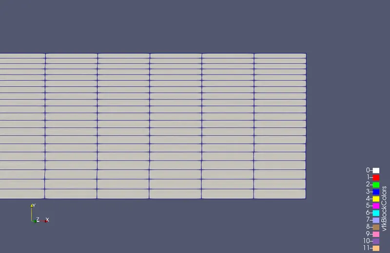
Mesh Generated
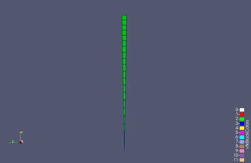
Front View
The grid spacing at the
Initial Conditions
Initial Velocity
The velocity at the inlet is specified and the at the outlet is specified as a gradient. The unit for velocity is specified using the 7 primary dimensions.
/*--------------------------------*- C++ -*----------------------------------*
  =========                 |
  \      /  F ield         | OpenFOAM: The Open Source CFD Toolbox
   \    /   O peration     | Website:  https://openfoam.org
    \  /    A nd           | Version:  8
     \/     M anipulation  |
*---------------------------------------------------------------------------*/
FoamFile
{
    version     2.0;
    format      ascii;
    class       volVectorField;
    object      U;
}
// * * * * * * * * * * * * * * * * * * * * * * * * * * * * * * * * * * * * * //

dimensions      [0 1 -1 0 0 0 0];

internalField   uniform (0 0 0);

boundaryField
{
    inlet
    {
        type            fixedValue;
        value uniform (0.1476 0 0);
    }

    outlet
    {
        type            zeroGradient;
    }

    top
    {
        type            fixedValue;
        value uniform (0 0 0);

    }

    bottom
    {
        type            empty;
    }

    front
    {
        type            wedge;
    }

    back
    {
        type            wedge;
    }
}

// ************************************************************************* //
Initial Pressure
The pressure at the inlet is not known and we specify is in form of a gradient. The outlet pressure is set to zero as the outlet pressure is the same as the atmosphere and the gauge pressure reading will be zero.
/*--------------------------------*- C++ -*----------------------------------*
  =========                 |
  \      /  F ield         | OpenFOAM: The Open Source CFD Toolbox
   \    /   O peration     | Website:  https://openfoam.org
    \  /    A nd           | Version:  8
     \/     M anipulation  |
*---------------------------------------------------------------------------*/
FoamFile
{
    version     2.0;
    format      ascii;
    class       volScalarField;
    object      p;
}
// * * * * * * * * * * * * * * * * * * * * * * * * * * * * * * * * * * * * * //

dimensions      [0 2 -2 0 0 0 0];

internalField   uniform 0;

boundaryField
{
    inlet
    {
        type            zeroGradient;
    }

    outlet
    {
        type            fixedValue;
        value uniform 0;
    }

    top
    {
        type            zeroGradient;
    }

    bottom
    {
        type            empty;
    }

    front
    {
        type            wedge;
    }

    back
    {
        type            wedge;
    }
}

// ************************************************************************* //
Fluid Properties
Based on the fluid properties are specified in the transport properties file. Here we assume the fluid to be water.
/*--------------------------------*- C++ -*----------------------------------*
  =========                 |
  \      /  F ield         | OpenFOAM: The Open Source CFD Toolbox
   \    /   O peration     | Website:  https://openfoam.org
    \  /    A nd           | Version:  8
     \/     M anipulation  |
*---------------------------------------------------------------------------*/
FoamFile
{
    version     2.0;
    format      ascii;
    class       dictionary;
    location    "constant";
    object      transportProperties;
}
// * * * * * * * * * * * * * * * * * * * * * * * * * * * * * * * * * * * * * //

nu              [0 2 -1 0 0 0 0] 8.9256e-07;


// ************************************************************************* //
Runtime and Timestep
Until now we have specified all the initial, boundary and fluid properties for the simulation setup. The staring and the ending time of the simulation along with the timestep are entered in the controlDict in the system folder.
The total time for the simulation is estimated on the basis of the domain length and how fast the information is travelling in the domain, and the time step is estimated using the CFL number based on the stability of the governing equation.
/*--------------------------------*- C++ -*----------------------------------*
  =========                 |
  \      /  F ield         | OpenFOAM: The Open Source CFD Toolbox
   \    /   O peration     | Website:  https://openfoam.org
    \  /    A nd           | Version:  8
     \/     M anipulation  |
*---------------------------------------------------------------------------*/
FoamFile
{
    version     2.0;
    format      ascii;
    class       dictionary;
    location    "system";
    object      controlDict;
}
// * * * * * * * * * * * * * * * * * * * * * * * * * * * * * * * * * * * * * //

application     icoFoam;

startFrom       startTime;

startTime       0;

stopAt          endTime;

endTime         15.81;

deltaT          0.0058;

writeControl    timeStep;

writeInterval   20;

purgeWrite      0;

writeFormat     ascii;

writePrecision  6;

writeCompression off;

timeFormat      general;

timePrecision   6;

runTimeModifiable true;


// ************************************************************************* //
Results
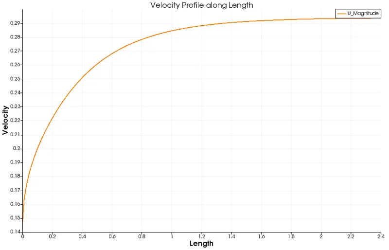
Each fluid particle moves at a constant axial velocity along a streamline and the velocity profile u(r) remains unchanged in the flow direction. There is no motion in the radial direction, and thus the velocity component in the direction normal to the pipe axis is everywhere zero. There is no acceleration since the flow is steady and fully developed.
Analytical Proof
%Entry Length for Laminar Flow

%Given Inputs
re=2100;    %Reynolds Number

%Assumptions
d=0.0254/2;     %Diamter of the Pipe
r=d/2;          %Radius of the Pipe

l_entry=0.05*re*d  %x-direction or flow direction

l_entry = 1.3335
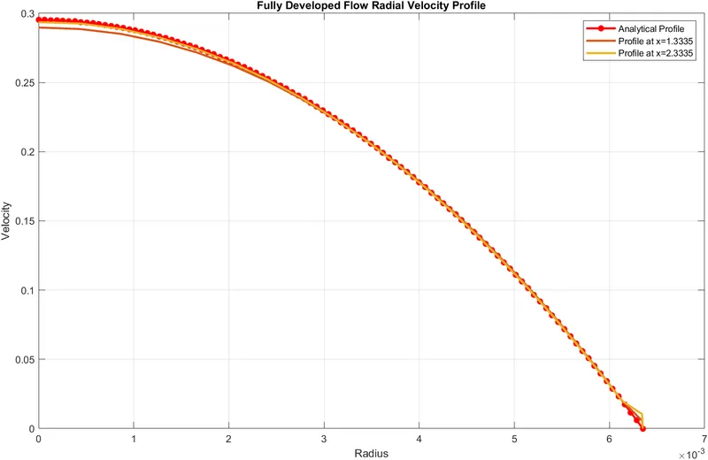
It is seen that after the hydrodynamic length the velocity along the length becomes constant.
The same can be seen in the below which compares the Radial Velocity profile of Fully Developed Flow Profiles.
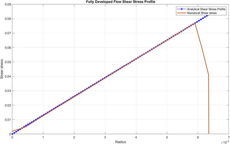
The shear stress at the pipe wall is related to the slope of the velocity `tau` profile at the surface. Noting that the velocity profile remains unchanged in the hydrodynamically fully developed region, the wall shear stress also remains constant.
The wall shear stress is the highest at the pipe inlet where the thickness of the boundary layer is smallest and decreases gradually to the fully developed value. Therefore, the pressure drop is higher in the entrance regions of a pipe and the effect of the entrance region is always to increase the average friction factor for the entire pipe.
%Analytically Calculating Shear Stress and Velocity Profile
R = linspace(0,(d/2),101);

for i = 1:length(R)
    tau(i) = 2*mu*v_max*(abs(R(i)))/r^2;
    u(i)=2*v_avg*(1-(R(i)^2/r^2));
end

%Shear Stress Profile
figure(2)
plot(R,tau,'b*-','LineWidth',1)
hold on
tau_23335=readmatrix('Tau_2.3335.csv');
plot(tau_23335(:,1),tau_23335(:,2),'LineWidth',2)
xlabel('Radius')
ylabel('Shear stress')
grid on
legend ('Analytical Shear Stress Profile','Numerical Shear stress')
title('Fully Developed Flow Shear Stress Profile')

%Velocity Profile
figure(3)
plot(R,u,'r*-','LineWidth',2)
hold on
v_13335=readmatrix('U_x13335.csv');
v_23335=readmatrix('U_x23335.csv');
plot(v_13335(:,1),v_13335(:,2),'LineWidth',2)
plot(v_23335(:,1),v_23335(:,2),'LineWidth',2)
legend('Analytical Profile','Profile at x=1.3335','Profile at x=2.3335');
xlabel('Radius')
ylabel('Velocity')
title('Fully Developed Flow Radial Velocity Profile')
grid on
Pressure Drop
A pressure drop due to viscous effects represent an irreversible pressure loss, and it is sometimes called pressure loss.
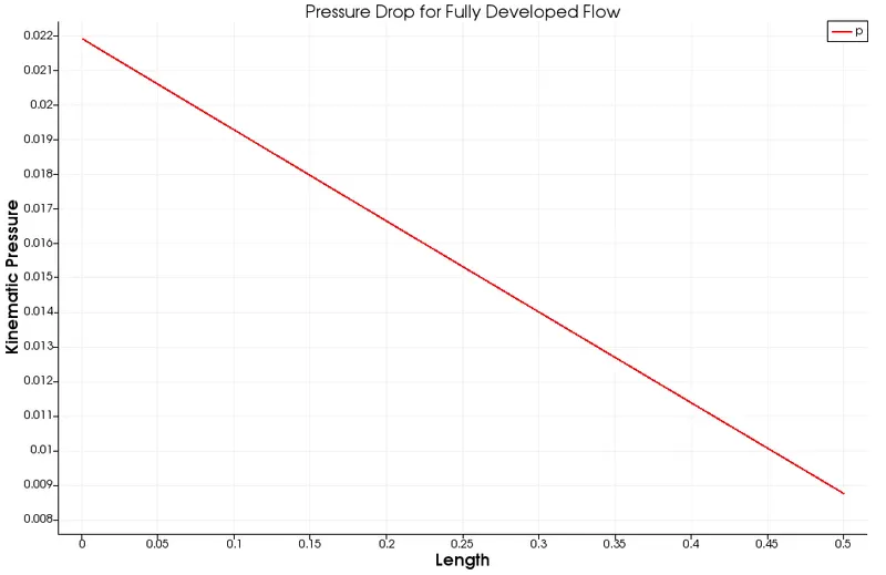
Numerical Pressure Drop from above graph=`0.022-0.0088=0.0132`
Analytical Pressure Drop
% Dynamic viscosity
mu = 0.89e-3;
% Density
rho = 997;

% Hagen poiseuille flow equations
v_avg = (re*mu)/(rho*d);
v_max = 2*(v_avg);

%Pressure Drop in Fully Developed Flow
del_p = (8*mu*0.5*v_avg)/(r^2);     %Pressure Drop
kinematic_p = del_p/rho;            %Kinematic Pressure Drop

del_p =

   13.0321


kinematic_p =

    0.0131