Week 11: FSAE Car Project

AIM:

• To run an aerodynamic flow simulation over an FSAE car in two phases. The first step is to configure a coarse simulation. This should be done in two cases for the second phase: one with the car travelling through many turns and another with the vehicle travelling on a straight road.

OBJECTIVE:

• Phase 1: Importing the geometry, cleaning up any errors, flagging appropriate surfaces as boundaries, creating a wind tunnel for the car with a ground surface, and ensuring the mentioned are correct by running a no-hydro simulation are all part of this phase.

• Phase 2: A hypothetical request from a racing company to produce a detailed report on the total downforce acting on the individual components of the car for two races is used in this phase.

THEORY:

1. FSAE model:

• SAE International organises the Formula SAE student design competition (previously known as the Society of Automotive Engineers, SAE). After a previous asphalt racing competition proved unsustainable, the SAE student branch at the University of Texas at Austin founded the competition in 1980.
• Formula SAE is based on the idea that a fictional manufacturing company has hired a student design team to create a small Formula-style race car. The prototype race car will be evaluated for commercial viability. The non-professional weekend autocross racer is the race car's target marketing group. Each student team designs builds and tests a prototype based on a set of rules, the goal of which is to ensure on-track safety (the students themselves drive the cars) while also encouraging creative problem-solving.

2. Down-force:

• Downforce is a downward lift force produced by a vehicle's aerodynamic features. If the vehicle is a car, the purpose of downforce is to increase the vertical force on the tyres, resulting in more grip. The purpose of the downforce on the horizontal stabiliser on a fixed-wing aircraft is to maintain longitudinal stability and allow the pilot to control the aircraft in pitch.

CASE SETUP:

PHASE - 1:

• The (Geometry. stl) was imported into Converge Studio.
• The diagnostic tool was used to detect open edges, intersection edges, and other errors such as orientation errors. Many features, such as 1. deleting the edge, node, and face were used to repair the geometry. 2. Using the patch tool to repair the edge 3. Stitching the two misaligned edges together.
• The geometry was scaled using the proper scale because it was created in Inch, so it was converted to Metre using the Scale feature.

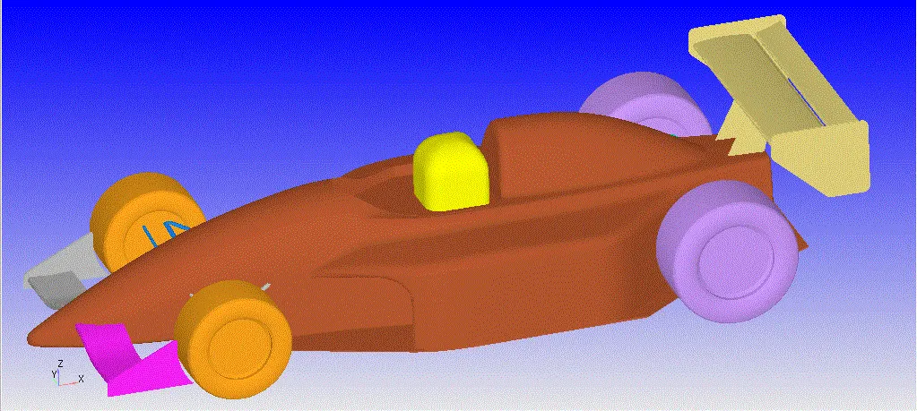
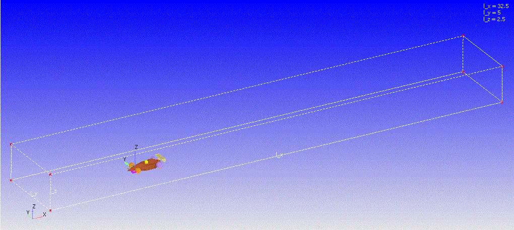
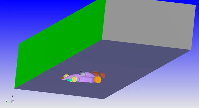
• The Virtual wind tunnel was created after the geometry was cleaned.
• The distance behind the FSAE car is approximately ten times the car's wheelbase.
• The distance in front of the FSAE car was calculated to be approximately four times the car's wheelbase.

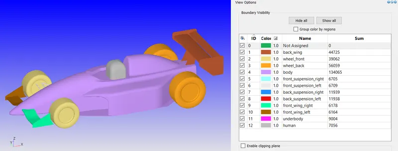
• The boundary tag was created after the Geometry and Wind Tunnel Geometry were created, along with different boundary IDs and colouring. A total of 16 different boundary tags were created for the geometry's multiple split triangles, with each face split into multiple triangles. The "Boundary" command in the "Geometry" dock was used to name the boundaries, and then the faces were assigned to appropriate tags along with id.

• Application Type: To run a steady-state simulation, first select a "Time-based" simulation under the Application type in the setup tree.
• Materials: The material tab was set to "Gas simulation" and "Air" as a predefined mixture.Air: Gas
• Fixed value for global transport parameters, The following value is used by default.
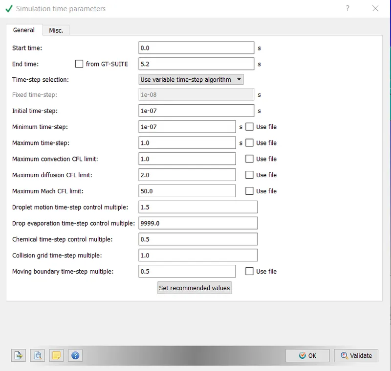
• Simulation Time parameters: This case study was run with the Transient solver and a "Density-based" solver.

Calculation:

• 32.5m horizontal length
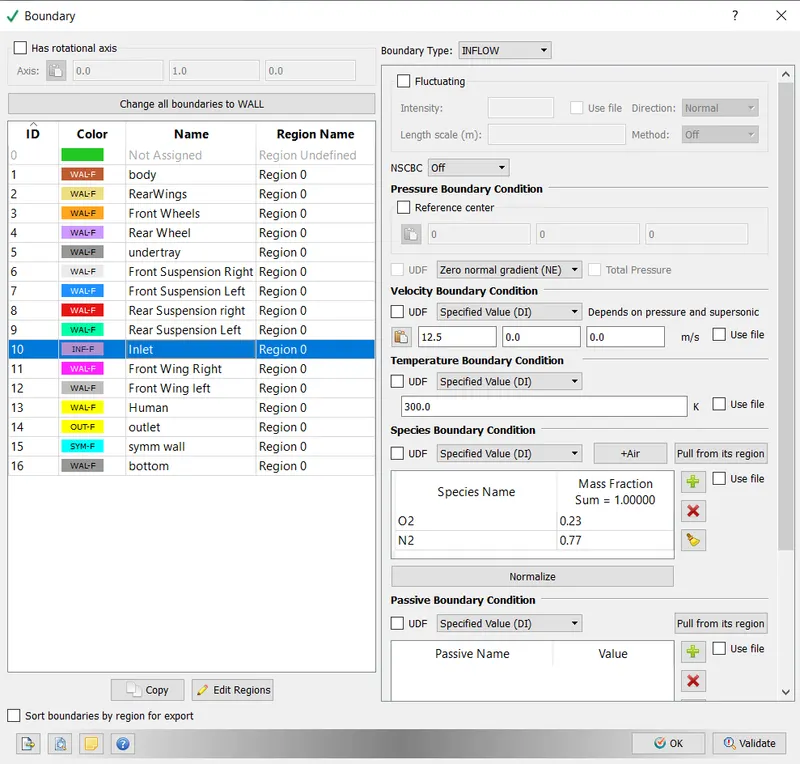
• Case 1's average velocity is 12.5m/s.
• Case 2's average velocity was 20.83m/s.
• Speed=Distance/time
• As a result, Time=2.6 sec
• We are simulating roughly 2 times of flow through time which is 5.6 s

• Boundary conditions: Inlet,

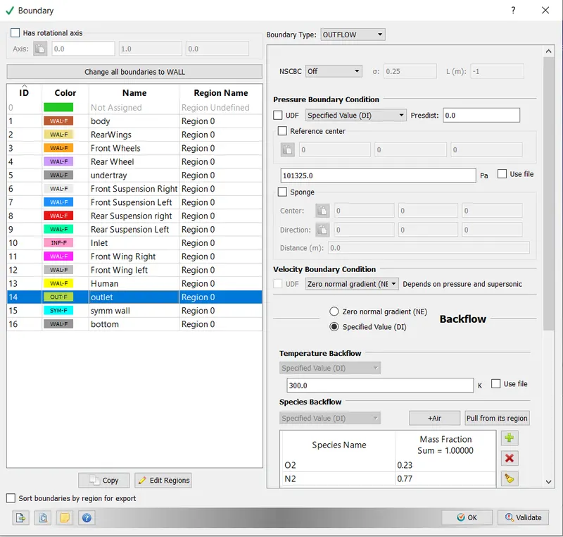
• Outlet:

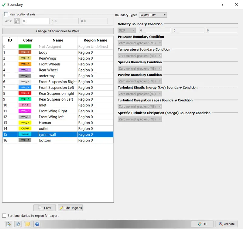
• Symmetry:

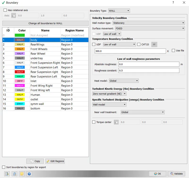
• Body:

• Physical models: Out of all the models, a turbulent model was chosen. The RANS standard K-omega SST model was selected.
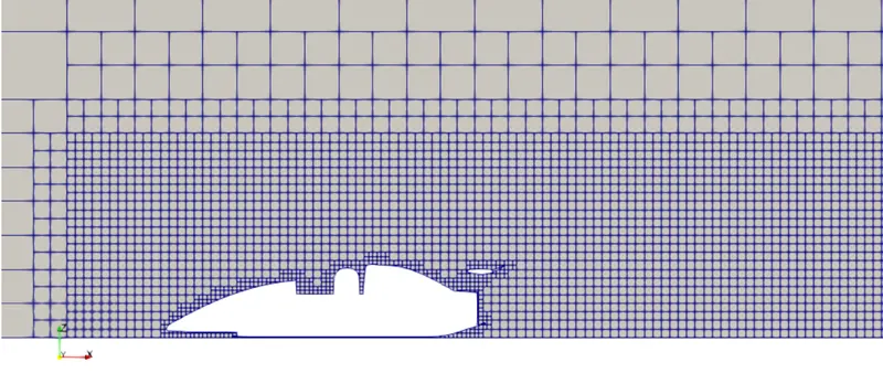
• Base grid: Due to limited computational resources, the case study was run with a coarse mesh grid size. Base mesh sizes are as follows:

S.No.	Dx(m)	Dy(m)	Dz(m)
1	0.5	0.5	0.5

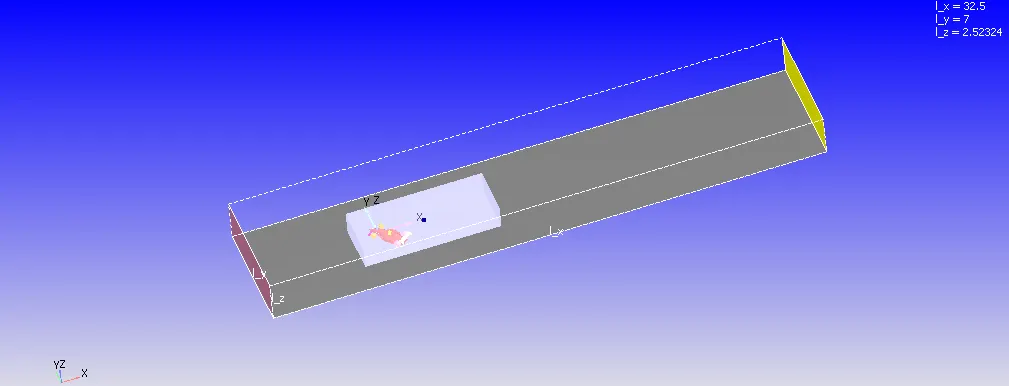
• Fixed Embedding: Fixed embedding was used to capture more cells near the throttle and obtain more precise data.

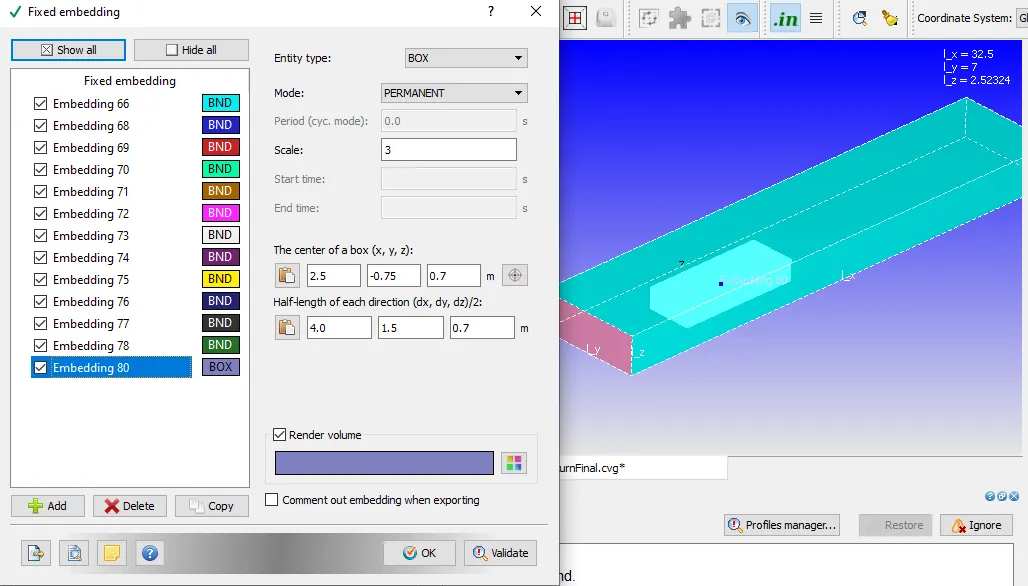
• Wind tunnel with a box embedded inside with finer computational cells to capture more data with greater precision.

• Output / Post-processing: The value of velocity in regions and initialization should be the same as the value of Inlet velocity.
• Also, when configuring the case, ensure that wall output (BOUNDARIES ONLY) is enabled, as this will dump wall-averaged output data, which is critical for any external aerodynamic simulations.
• Existing value post-variable selection
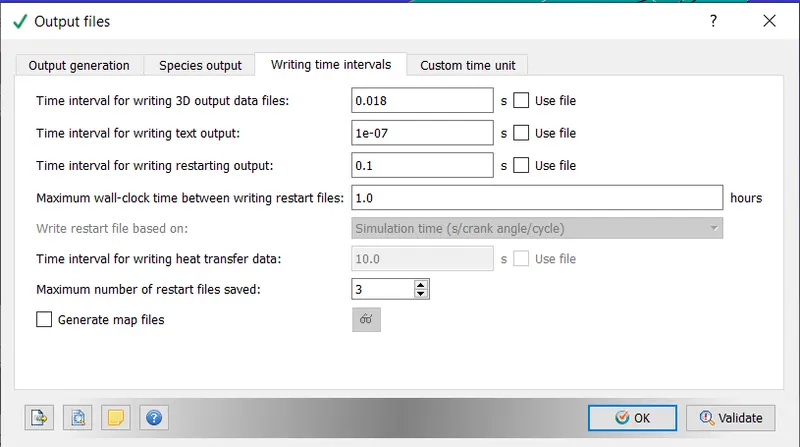
• Output Files- 0.018 s time interval for writing 3D output files -0.1s is the time interval for writing restart files.

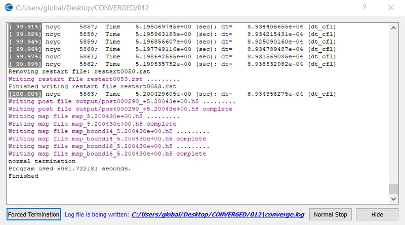
• Completed Calculation: Phase 1:

PHASE -1 RESULT:

• MESH:

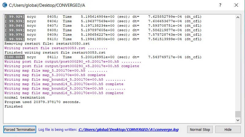
• The simulation runs successfully:

CASE SETUP PHASE - 2:

• Case- 1 The situation occurred while turning.
• Racetrack conditions - Lot of turns

The average lap speed is 45kmph, with 70% of turns being at 45 degrees.
20% turns at an angle of 80 degrees
10% turns at a 20-degree angle
The model of the car was rotated along the Z-axis.

• This is the car seen in the wind tunnel (some surfaces hidden):

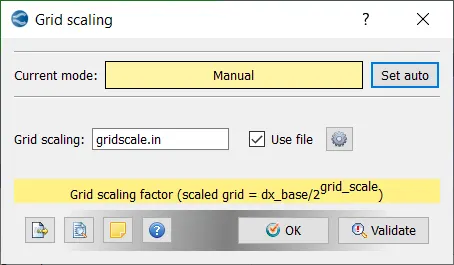
• All the default settings remain the same except the base grid and here we are adding a grid scale for accurate scaling.
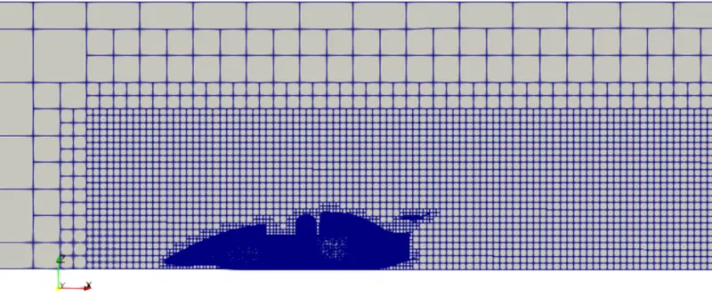
• Base grid: Fixed Embededding and Grid Scaling have been enabled to ensure that a finer mesh is used in regions close to the car's body.
• This value was chosen to ensure that the boundary fixed embedding generates a mesh that accurately captures the boundary layer at the car's surface. The yplus value must be between 1 and 100 for this. With 1-5 representing the viscous region, 5-30 representing the buffer region, and greater than 30 representing the log-law region. The mesh size for the K-omega turbulence model should be chosen so that the smallest mesh lies in the log-law region. (yplus > 30). Also, the value of yplus cannot be too high, or the simulation will lose accuracy and become invalid. Ideally, the value of yplus should be between 30 and 100.
• According to the yplus calculator here: https://www.pointwise.com/yplus/index.html, the final cell size for a yplus of 60 should be at least 1.8mm for the current flow conditions, for the final grid size to be 1.8mm, and embed scale to be no greater than 5. (greater than 5 or 6 causes load balancing because all processors have to communicate with each other more often.

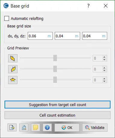
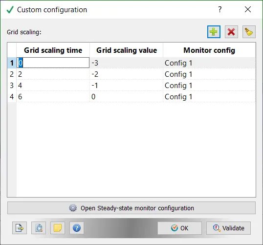
• Grid-scale: To ensure the simulation runs faster during the early stages of the flow, an additional grid scaling factor was introduced. This ensures that fewer resources and time are used for in-simulation times when no useful data is generated.

RESULT: (Case 1- A lot of turns):

• The geometry is rotated from its initial position (parallel to side planes) in an angle that varies between the three cases here (45,80,20)

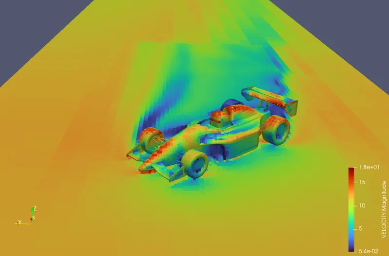
• VELOCITY CONTOUR:

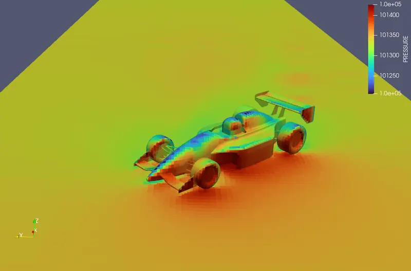
• PRESSURE CONTOUR:

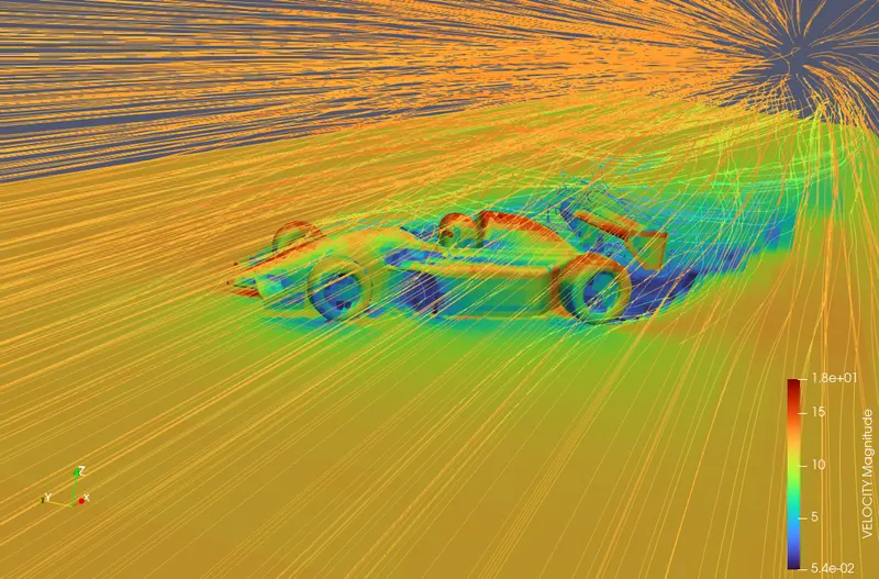
• STREAM VELOCITY:

• Drag and lift CALCULATION:

Pressure forces:

Boundary ID	Name	Pressure force in the X-direction	Pressure force in the Y-direction
1	Body	3814.63	37.54
2	Rear wing	3.61	-6.30
3	Front wheels	9.65	-3.21
4	Rear wheels	8.34	-2.27
5	Front wing right	-101.4	187.32
6	Front wing left	182	-101
7	Front suspension right	8.8	-2.5
8	Front suspension left	-3.61	-9.59
9	Front suspension right	-9.7	-19.37
10	Rear suspension right	-19.81	-9.60

Observation:

• We can see from the velocity contours above that there is more wake region on the backside.
• More pressure is applied to the side of the car body that faces the flow.
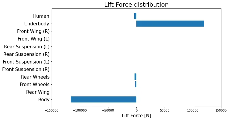
• The rear wing generates a negative lift, which improves the car's movement and grip. This area of the car also has less drag.
• Negative lifts are also produced by the front wheels, which are followed by the rear wheels.
• The left front wing experiences more negative lift and the tyres require more grip at this point because the car is turning. As a result, the front wing of a car has a significant property when turning.
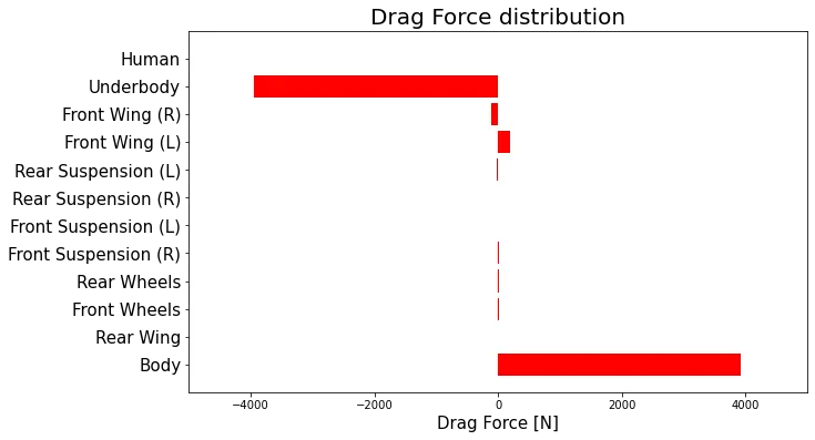
• Because the car is turning, the drag force it encounters is greater because the frontal area of the car is larger.

The average drag force on various FSAE car components:

The average lift force on various FSAE car components is:

RESULT: (Case 2- Straight road):

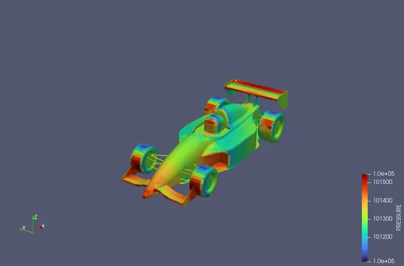
• VELOCITY CONTOUR:

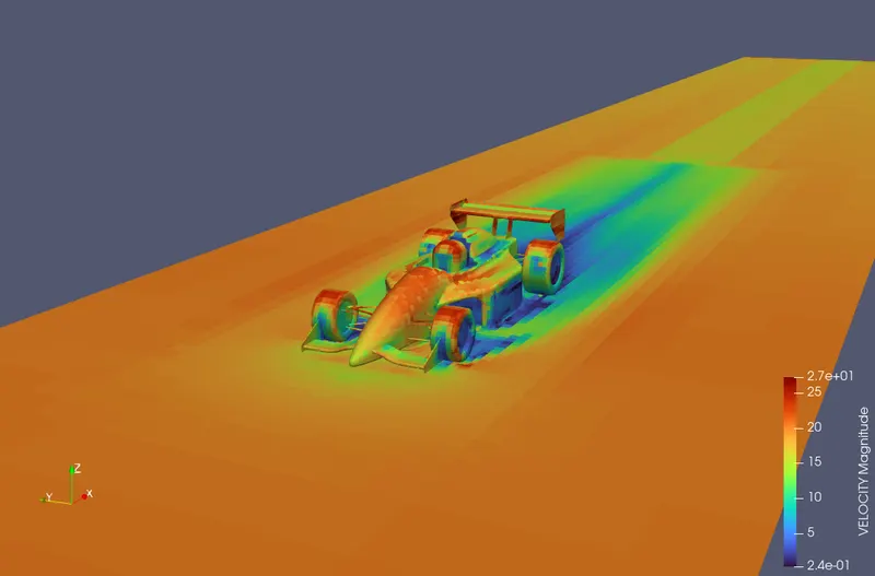
• PRESSURE CONTOUR:

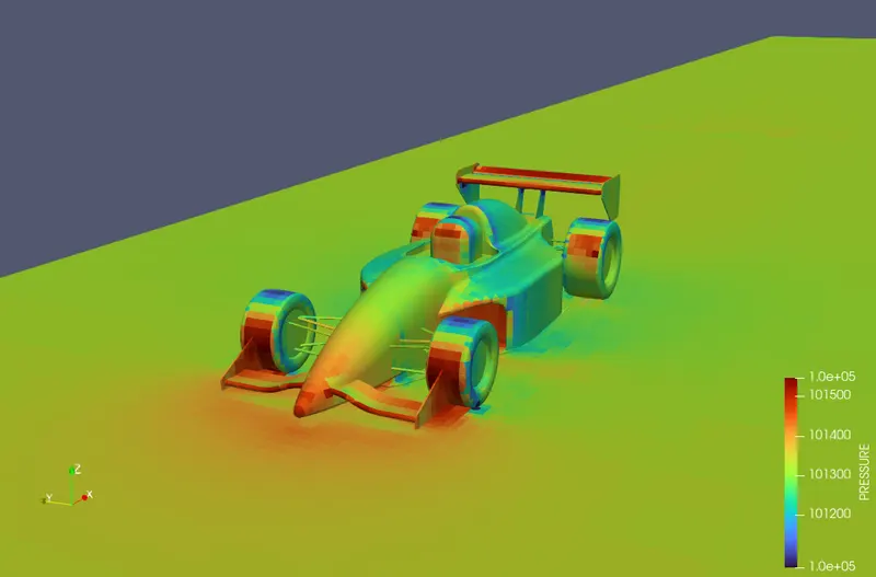
• STREAM VELOCITY:

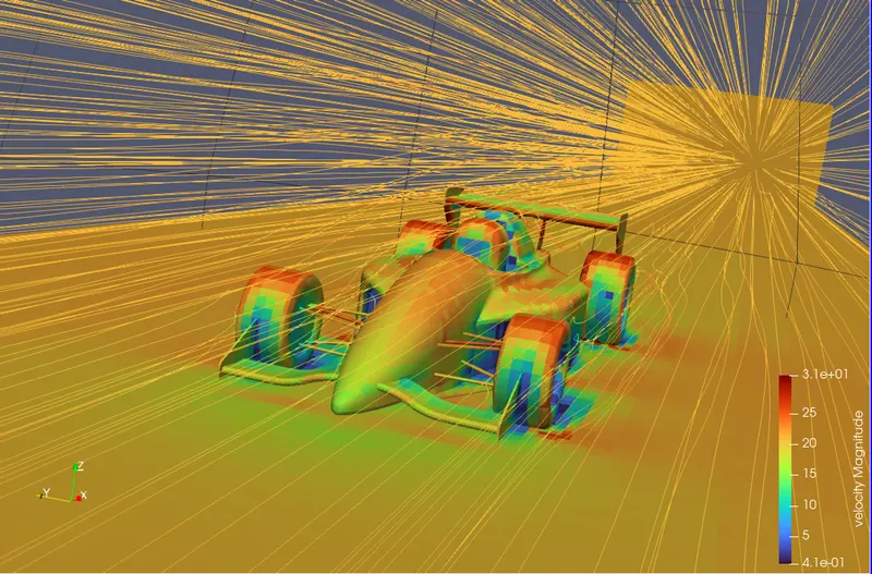
• Drag and lift:

Pressure forces:

Boundary ID	Name	Pressure force in the X-direction	Pressure force in Y-direction
1	Body	5781	0.49
2	Rear wing	1.1	-0.12
3	Front wheels	-5.78	2.274
4	Rear wheels	-4.17	0.112
11	Front wing right	-61.83	-267
10	Front wing left	-60.12	-295
6	Front suspension right	-4.27	8.84
7	Front suspension left	-4.16	8.33
8	Rear suspension right	21.58	7.89
9	Rear suspension left	21.29	7.25

Observations:

• The velocity contours show that there are fewer velocity fluctuations around the car. The pressure is distributed more at the front than at the back.
• Here, too, the front wings produce more negative lift, assisting the car in remaining firmly planted on the ground.
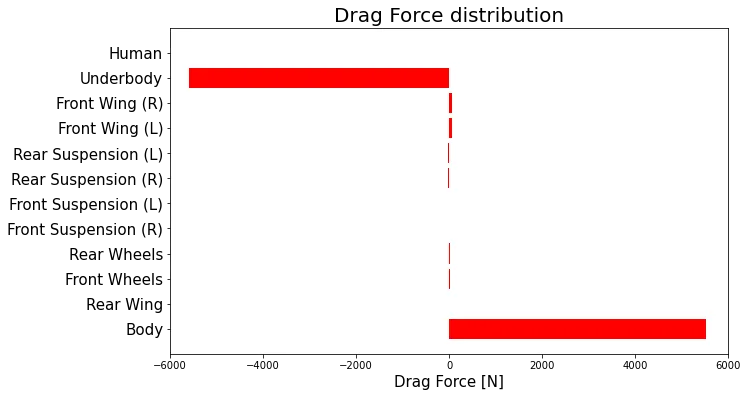
• The body is subjected to more drag.
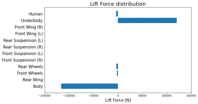
• The rear wing also produces negative lift, but it is significantly less than the frontal wings.
• In this case, the size of the wake region is smaller than in the first.
• Making the car body more streamlined can help to reduce drag and the size of the wake region.
• If the negative lift is required at the back, the rear wings should be tilted upwards to avoid allowing drag to take over.

Drag force averaged across various FSAE car components:

The average lift force on various FSAE car components:

CONCLUSION:

• In Phase 1, a trial case with coarse mesh was created and tested successfully.
• The second phase is set up with more mesh detailing and an efficient setup.
• The Y+ values have yet to reach the desired level, indicating that more computational resources are required.
• Two cases were included in the second phase.
• The velocity contours, pressure contours, drag force values, and lift force values were extracted.
• Drag and lift forces fluctuate in a cyclic fashion over time.