Week-11 Challenge: Braking
1) For a defined driving cycle, calculate the energy required for braking.
riving Cycle: A driving cycle are a set of vehicle speed points versus time, it is used to calculate the fuel consumption of a vehicle, which is later on is compared with different vehicles. Main use of driving cycle are as follows:
- To assess the performance of a vehicle (fuel economy, emission tests)
- To analyze battery state and energy consumption in Electric Vehicles
- To simulate vehicle model prior to the actual development
Braking: Road vehicles involves the conversion of kinetic energy into thermal energy (heat). When stepping on the brakes, the driver commands a stopping force several times as powerful as the force that puts the car in motion and dissipates the associated kinetic energy as heat.
The process of braking follows the law of conservation of energy i.e. Energy cannot be created or destroyed it can only be converted into another form.
E(kinectic) = 1/2*m*v^2...
where,
m = mass of the vehicle in Kg
v = velocity of the vehicle in m/s
E(kinectic) = Kinectic energy in KJ
In our case, velocity will be (V-Vi) where, V is the speed of the vehicle, Vi the speed of the vehicle which is slow down or brought down to rest.
Matlab Code for calculating Energy required for Braking
clear all
close all
clc
%Read the Drive Cycle data from given .xls file
DC=xlsread('VelocityandTime.xlsx');
T=DC(:,1); %Time in seconds
S=DC(:,2); %Speed in Kmph
%other data
m = 1000; %mass in Kg
V=S./3.6; %Speed in m/s
%To create an Array to store values for Deceleration & Braking Energy
Z=length(T);
deceleration=zeros(1,Z);
acceleration=zeros(1,Z);
BE=zeros(1,Z);
AE=zeros(1,Z);
for i=1:(length(T)-1)
if V(i)>V(i+1)
BE(i)=0.5*(V(i)-V(i+1))^2; %Braking Energy in Joules
speed_decrease(i)=V(i+1)-V(i);
deceleration(i)=speed_decrease(i);
%since Time Delta is 1s Acc/dec=V/T..m/s^2, where T=1
end
if V(i)<V(i+1)
AE(i)=0.5*m*(V(i)-V(i+1))^2; %Accelerating Energy in Joules
speed_increase(i)=V(i+1)-V(i);
acceleration(i)=speed_increase(i);
end
end
%Total Braking Energy in KJ
B_E=(sum(BE)/1000);
%Total Acceleration Energy in KJ
A_E=(sum(AE)/1000);
%Plotting Curves
figure(1)
subplot(2,1,1)
plot(T,S,'color','b')
xlabel('Time(s)')
ylabel('Speed(Kmph)')
title('Drive Cycle')
subplot(2,1,2)
plot(T,deceleration,'color','r')
hold on
plot(T,acceleration,'color','g')
xlabel('Time(s)')
ylabel('Acc/Dec(m/s^2)')
title('Acceleration-Deceleration')
figure(2)
plot(T,BE)
hold on
plot(T,AE)
xlabel('Time(s)')
ylabel('Energy(J)')
title('Energy consumed during Braking & required for acelerating throughout Drive Cycle')
legend('Braking Energy','Accelerating Energy')
fprintf('Total Energy consumed during Braking is %f KJ',B_E)
disp(' ')
fprintf('Total Energy consumed during Acceleration is %f KJ',A_E)
For Driving cycle an Excel sheet is imported,
| time | velocity |
| 1 | 0 |
| 2 | 0 |
| 3 | 0 |
| 4 | 0 |
| 5 | 0 |
| 6 | 0 |
| 7 | 0 |
| 8 | 0.45 |
| 9 | 0.46 |
| 10 | 0.47 |
| 11 | 0.47 |
| 12 | 0.48 |
| 13 | 0.49 |
| 14 | 0.496 |
| 15 | 0.503429 |
| 16 | 0.510857 |
| 17 | 0.518286 |
| 18 | 0.525714 |
| 19 | 0.533143 |
| 20 | 0.540571 |
| 21 | 0.548 |
| 22 | 0.555429 |
| 23 | 0.562857 |
| 24 | 0.570286 |
| 25 | 0.577714 |
| 26 | 0.585143 |
| 27 | 0.592571 |
| 28 | 0.6 |
| 29 | 0.607429 |
| 30 | 0.614857 |
| 31 | 0.622286 |
| 32 | 0.629714 |
| 33 | 0.637143 |
| 34 | 0.644571 |
| 35 | 0.652 |
| 36 | 0.659429 |
| 37 | 0.666857 |
| 38 | 0.674286 |
| 39 | 0.681714 |
| 40 | 0.689143 |
| 41 | 0.696571 |
| 42 | 0.704 |
| 43 | 0.711429 |
| 44 | 0.718857 |
| 45 | 0.726286 |
| 46 | 0.733714 |
| 47 | 0.741143 |
| 48 | 0.748571 |
| 49 | 0.756 |
| 50 | 0.763429 |
| 51 | 0.770857 |
| 52 | 0.778286 |
| 53 | 0.785714 |
| 54 | 0.793143 |
| 55 | 0.800571 |
| 56 | 0.808 |
| 57 | 0.815429 |
| 58 | 0.822857 |
| 59 | 0.830286 |
| 60 | 0.837714 |
| 61 | 0.845143 |
| 62 | 0.852571 |
| 63 | 0.86 |
| 64 | 0.867429 |
| 65 | 0.874857 |
| 66 | 0.882286 |
| 67 | 0.889714 |
| 68 | 0.897143 |
| 69 | 0.904571 |
| 70 | 0.912 |
| 71 | 0.919429 |
| 72 | 0.926857 |
| 73 | 0.934286 |
| 74 | 0.941714 |
| 75 | 0.949143 |
| 76 | 0.956571 |
| 77 | 0.964 |
| 78 | 0.971429 |
| 79 | 0.978857 |
| 80 | 0.986286 |
| 81 | 0.993714 |
| 82 | 1.001143 |
| 83 | 1.008571 |
| 84 | 1.016 |
| 85 | 1.023429 |
| 86 | 1.030857 |
| 87 | 1.038286 |
| 88 | 1.045714 |
| 89 | 1.053143 |
| 90 | 1.060571 |
| 91 | 1.068 |
| 92 | 1.075429 |
| 93 | 1.082857 |
| 94 | 1.090286 |
| 95 | 1.097714 |
| 96 | 1.105143 |
| 97 | 1.112571 |
| 98 | 1.12 |
| 99 | 1.127429 |
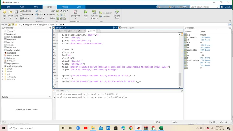
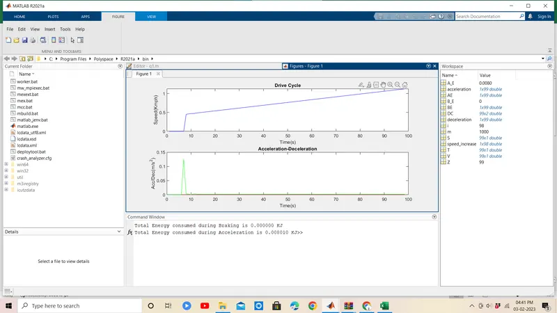
We can observe after the simulation is completed the two values Total energy required in braking 0.066975 KJ whereas, Total Energy consumed during Acceleration is 95.342400 KJ.
2) Why electric motor can’t develop braking torque at high speed similar to starting? How electric and mechanical brakes are coordinated?
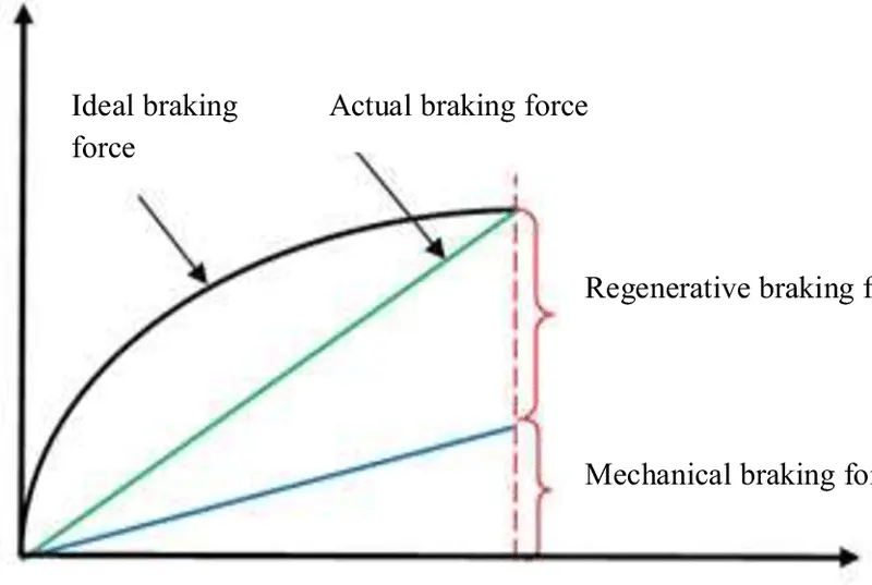
Mechanical Braking
Mechanical brakes are applied by brake shoes which are pressed with force against the wheel of the train. In mechanical braking, the braking force is generally produced by means of piston-cylinder arrangement. The movement of the piston is transmitted to the brake shoes through a system of levers.
Electric Braking
In electric braking, the kinetic energy of the moving parts of the motor is converted into electrical energy which is either dissipated in a resistor or returned to the supply source. Thus, electric braking is a system of braking in which a braking action is applied to an electric motor by causing it to act as a generator.
Comparison between Electrical Braking and Mechanical Braking
The following table highlights the points that differentiate an electrical braking system from a mechanical braking system −
| Point of Comparison | Mechanical Braking | Electrical Braking |
|---|---|---|
| Cost | The initial cost of mechanical braking is low. | Electrical braking has high initial cost. |
| Maintenance | Mechanical braking requires frequent maintenance as it produces excessive wear and tear of brake shoes. | Electrical braking requires very little maintenance because of absence of mechanical equipment. |
| Replacement of brake shoes | Due to excessive wear and tear, mechanical braking requires frequent replacement of brake shoes. | Electrical braking does not require replacement of brake shoes. |
| Maintenance cost | Due to constant wear and tear of brake lining, frequent adjustments are necessary to compensate the offset error, therefore maintenance cost of mechanical braking is high. | Electrical braking requires less maintenance and hence, its maintenance cost is low. |
| Production of metal dust | Mechanical braking produces metal dust which causes wearing of bearings. | In case of electrical braking, no metallic dust is formed. |
| Braking action | If the mechanical brakes are not correctly adjusted, then sudden braking action produces shock, which results in discomfort to passengers. | In electrical braking, the adjustment of braking system is easy and the braking action is gradual and smooth. |
| Heat production & its effect | In mechanical braking, heat is produced in brake shoes of brake lining, which may damage the brake lining and may result in failure of braking system. | In electrical braking, heat is produced at a convenient place which is not harmful to the braking system. |
| Regenerative braking | In mechanical braking, regenerative braking is not possible. | In electrical braking, 60% to 80% of kinetic energy of moving parts can be fed back to the supply line in regenerative braking. |
| Used alone or supplemented | Mechanical braking alone can be used. | Electrical braking is alone not sufficient, and it is supplemented by mechanical braking. |
| Holding torque | Mechanical braking is applied to hold the system at any position. | Electrical braking cannot produce holding torque. |
| Efficiency | Mechanical braking is less efficient due to excessive wear and tear. | Electrical braking is highly efficient. |
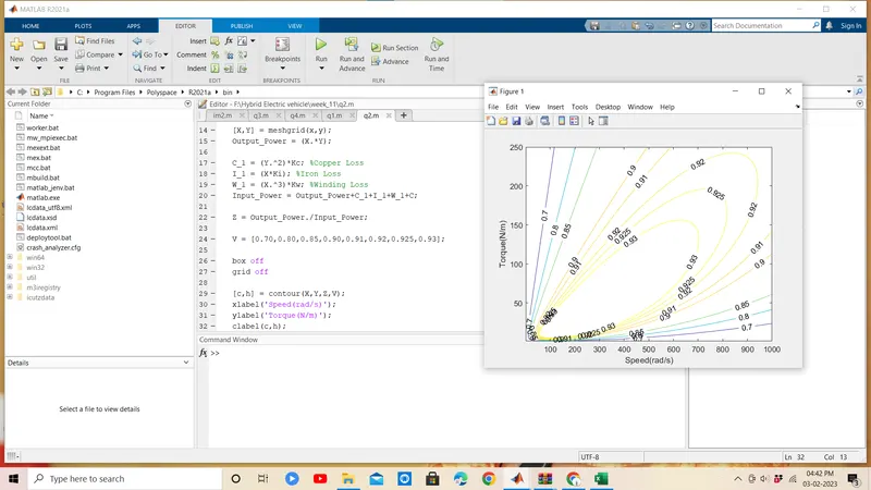
3) Make a MATLAB program which plots contour of given motor speed, torque and efficiency values. Attach the code as a .m file attach a screenshot of all the plots.
MATLAB Code:
%Efficiency Mapping for Electric Motors
clear all
close all
clc
x = linspace(1,1000); % Speed in rad/s
y = linspace(1,250); % Torque in Nm
%Motor loss constants
Kc = 0.2; %Copper Loss
Ki = 0.008; %Iron Loss
Kw = 0.00001; %Winding Losses
C = 20; %Constant Motor Losses
[X,Y] = meshgrid(x,y);
Output_Power = (X.*Y);
C_1 = (Y.^2)*Kc; %Copper Loss
I_1 = (X*Ki); %Iron Loss
W_1 = (X.^3)*Kw; %Winding Loss
Input_Power = Output_Power+C_1+I_1+W_1+C;
Z = Output_Power./Input_Power;
V = [0.70,0.80,0.85,0.90,0.91,0.92,0.925,0.93];
box off
grid off
[c,h] = contour(X,Y,Z,V);
xlabel('Speed(rad/s)');
ylabel('Torque(N/m)');
clabel(c,h);
Explanation:
In this MATLAB script, we create arrays for the speed and the torque of the motor using the ‘linspace’ command. For the speed, consider a range of values from 0 to 2000 radians per second whereas for the torque, consider a range of values from 0 to 300Nm.These arrays are then used to create 2D grid coordinates using the ‘meshgrid’ command. These coordinates will help in the creation of the contour plot. In order to find the efficiency of the motor, we need to consider the various losses that occur in the motor’s operation. These are:
Copper losses
Iron losses
Windage losses
Conduction losses
These various losses are dependent on the speed and the torque of the motor. They each also have a characteristic constant of proportionality which are all assumed for the following calculations and represented as 'K'. In each calculation, the speed and the torque are represented respectively as: ω and T.
Copper losses = KCu⋅ω2
Iron losses =KFe⋅T2
Windage losses =Kw⋅T3
The values of coefficients are taken as general values. Conduction losses are assumed to be 18 Joules.
Finally we plot the contour with the 'contour' command. In addition, an array for the efficiency values we want to plot for is created called 'W' and is assigned for values ranging from an efficiency level of 0.75 to 0.95. This array is used in the creation of the contour. Axis labels and a title is also made for better readability.