Week-11 Challenge: Braking

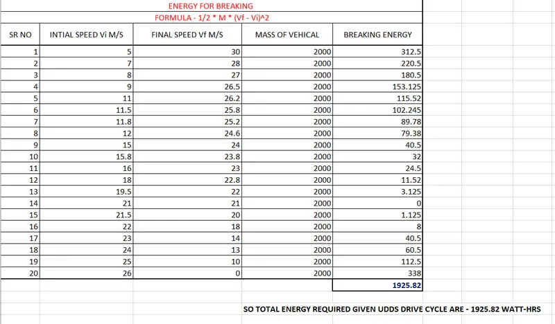
1 For a defined driving cycle, calculate the energy required for braking.

ans -

Driving Cycle -

A driving cycle is a series of data points representing the speed of a vehicle versus time.

Another use for driving cycles is in vehicle simulations. More specifically, they are used in propulsion system simulations to predict performance of internal combustion engines, transmissions, electric drive systems, batteries, fuel cell systems, and similar components.

There are two types of driving cycles:

1 -Transient driving cycles involve many changes, representing the constant speed changes typical of on-road driving.

2 - Modal driving cycles involve protracted periods at constant speeds.

Energy Required for breaking -

To accelerate a vehicle we need some Energy to accelerate, like the same to brake the vehicle we need some energy to brake.

1 - In acceleration the velocity changes from initial to final velocity value. While Braking the velocity changes from Final value to initial value or 0.

2 - So, in this case of Braking, the Kinetic Energy is given by,

Braking Energy = 1/2 * M * (Vf - Vi)^2

where M - Mass of the vehicle

Vi - Initial velocity

Vf - Final velocity

When using this formula calculating breaking energy so we are generate the exls file to given in 20 break point with constant vehicle load .

2 Why electric motor can’t develop braking torque at high speed similar to starting? How electric and mechanical brakes are coordinated?

ans -

Regenerative braking –

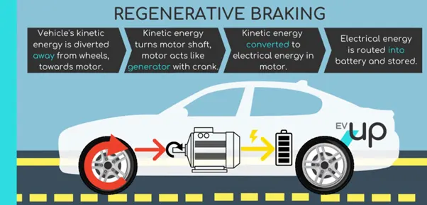
Regenerative braking is a mechanism found on most hybrid and full-electric vehicles. It captures the kinetic energy from braking and converts it into the electrical power that charges the vehicle’s high voltage battery. Regenerative braking also slows the car down, which assists the use of traditional brakes.

In a conventional braking system, a car slows down due to friction between the brake pads and rotors. But this system is highly inefficient when it comes to conserving energy. Nearly all of the kinetic energy propelling your car forward is lost as heat when you apply the brakes. That’s a lot of wasted energy!

Regenerative braking solves this problem by recapturing upwards of 70% of the kinetic energy that would otherwise be lost during braking. The amount of energy recovered depends on your car model and driving behaviour.

There are some limits to regenerative braking. For starters, it can only recapture the energy used to accelerate the vehicle or climb an incline, minus some inevitable losses. Speaking of which, the energy recaptured by regenerative has to go through the full conversion process – from chemical to electrical to mechanical to road – twice. Typical efficiencies for each major step in this process are 99% for lithium chemistry batteries, 96-98% for inverters, 80-95% for motors (though this can drop much lower, especially at either extreme of the power range), 95% for hypoid gear differentials (which tends to get overlooked) and, finally, 85-95% for tires. Even taking the best-case values for each figure, that comes out to an overall efficiency from battery to road of 83%, and a round-trip efficiency of 69%; in other words, you can’t always regenerative brake your way to longer range.

Another, more obvious, limit to regenerative braking is tire adhesion. This is less of an issue in front-wheel drive EVs, but applying too much braking torque to the rear wheels in rear- or all-wheel drive EVs (especially motorcycles) can, shall we say, make for an exciting driving experience. This is due to the phenomenon called “load transfer,” in which the center of mass on any wheeled vehicle shifts due to acceleration or deceleration forces, and this shift is proportional to the height of the center of mass above ground and inversely proportional to the wheelbase (note that in a 4-wheel vehicle, load transfer can occur front to back, as during acceleration and braking, or side to side, as during turning). Load transfer can beexacerbated by weight transfer, which is the same effect except caused by suspension travel or actual shifting of liquids, cargo, etc, in the vehicle. Together these phenomena lower the weight over the rear wheels during braking, making them less effective at transferring force without skidding.

The maximum torque from regenerative is generally the same as during motoring, and while this torque can be impressive, it still isn’t anywhere close to what the mechanical brakes can achieve, thus regenerative cannot substitute for the mechanical brakes. The equation to calculate the effective power of the brakes to decelerate a given weight at a given g-force is no different from its more familiar use in acceleration -

P = m * a * v

where P is in Watts, m is weight in kg, a is acceleration in m/s2, and v is velocity in m/s. For example, the 2019 Audi e-tron Quattro has an estimated weight of 2,400 kg, and should be easily capable of braking at 0.8 g of deceleration (1 g = 9.81 m/s2); if traveling at 100 kph (62 mph, 27.78 m/s), that works out to a brake power of 523 kW. Compare that to the estimated maximum power output of its electric drivetrain of 300 kW. There is a flip side to this as well: using regenerative to decelerate at too low of a rate might not produce enough power to overcome the losses in the electrical components of the drivetrain. As crazy as it might seem, this would lead to regenerative actually decreasing range compared to mechanical braking. This is because the electrical components incur little to no loss when the motor is not active (either motoring or generating) – there are no resistive losses in the battery or wiring, no switching and conduction losses in the inverter, no iron and copper losses in the motor – but once the motor is put into operation all of those losses come into play. Nailing down exact numbers for these losses is notoriously difficult, but a reasonable range would be 5-20 kW for just the electrical components (higher for heavier/higher-power/less-efficient vehicles). Dropping the rate of deceleration in the above example to 0.01 g would result in ~6.5 kW of power from regenerative, but if the combined electrical losses are, say, 8 kW, then ~1.5 kW of extra drain on the battery will occur.

Similarly, once speed drops below a certain point, regen will fail to return enough energy to be worth the bother even if the rate of deceleration is high. The kinetic energy equation:

Ke = 0.5 * m * v2

where Ke is in joules (or watt-seconds), m is weight in kg, and v is velocity in m/s, shows that energy drops off dramatically with decreasing velocity. A 2,400 kg vehicle traveling at 100 kph has 926 kJ (0.26 kW-hr) of recoverable energy, but at 10 kph that drops to a paltry 0.0026 kW-hr, or 100 times less. Even with no losses to contend with that’s a mere 2.6 watt-hours of energy. Even if decelerating at a sufficient rate to produce more power than the electrical losses, that’s not exactly worth writing home about. Still, regen is a net positive most of the time, and something ICE vehicles can’t do at all.

Electric motor can’t develop braking torque at high speed similar to starting, because Braking torque is applied in the opposite direction of the rotation. We can use a mechanical brake to produce a braking torque. We can also do it electrically.

How electric and mechanical brakes are coordinated –

Mechanical Braking

Mechanical brakes are applied by brake shoes which are pressed with force against the wheel of the train. In mechanical braking, the braking force is generally produced by means of piston-cylinder arrangement. The movement of the piston is transmitted to the brake shoes through a system of levers.

Electric Braking

In electric braking, the kinetic energy of the moving parts of the motor is converted into electrical energy which is either dissipated in a resistor or returned to the supply source. Thus, electric braking is a system of braking in which a braking action is applied to an electric motor by causing it to act as a generator.

Regenerative braking can recover and reuse braking energy, which is an important characteristic of electric vehicles(EV). But it also has a negative impact on the control of anti-lock braking system(ABS). For the purpose of recovering energy efficiently, the constraints of braking force distribution between front and rear axle was analyzed, and then a regenerative braking distribution strategy was determined. The anti-lock control of the mechanical braking system was analyzed based on logic threshold method. To reduce the influence on ABS, the motor regenerative braking force was controlled to decrease rapidly as soon as ABS started. The simulation results show that the braking force control strategy used in this paper can recover energy adequately, ABS can work properly and coordinate with regenerative braking system when emergency braking.

Electric and mechanical brakes are coordination There are two brake control strategies namely, SERIES & PARALLEL. SERIES Brakes will be applied one after the another so which they are connected in series

Series control break system –

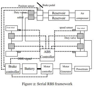
The drive train for the bus includes an Auxiliary Power Unit (APU) which consists of an internal combustion engine coupled to a generator and rectifier that can power the electric motor or charge the batteries as requested by the Vehicle Control Unit (VCU). The electric motor, which is controlled by the motor control unit, can work as a drive motor or a generator. The battery can drive the motor or absorb the current from APU and from the electric motor when the motor is working as a generator during regenerative braking. The framework of the series RBS shown in Figure 2 consists of the RBS control unit, the ABS system, and two duty valves used to adjust friction braking force. The duty valves are installed in the front and rear brake lines. The duty valves, which are also used in the ABS, are proven and have a quick response time. The different states of the two valves will determine the air pressure in the brake chambers. The brake control unit sends PWM signals to the valves to control the pressure, thereby controlling the mechanical braking force under the command of the control system of the RBS. When the ECU detects a rear wheel lockup, the ABS controller emits a signal to activate the modulator valve which will cause the brakes to pulsate, thereby mitigating the wheel lockup condition. Since the RGS is installed on the rear axle, the same signal can be used to control the regenerative braking force and thereby improve vehicle stability by minimizing wheel lockup during hard braking operations.

Parallel Brake Control or Parallel RBS –

In this type of brake control system both the Mechanical Brakes and RBS are applied simultaneously.

The machines which run on ac supply are called AC machines. The rotating machines in ac supply are called AC motors. The losses in ac motors are mainly classified into two types:

1. Constant losses: The losses which are constant all the time in the machine are called constant losses. These losses are further divided as –

Constant Losses - This is denoted as C.

1. Core losses: The losses that occurred due to constant flux density in the core are called core losses. These losses are the addition to both hysteresis and eddy current losses.

Copper losses = kc⋅T^2

1. Mechanical losses: The losses that occurred due to rotating parts are called mechanical losses. These losses change according to the speed of the motor. These losses are classified into two types such as friction and windage losses.

Windage Losses = kw⋅ω^3

1. Iron Losses - Iron Losses are nothing but Magnetic losses, which is denoted as ki⋅ω, where ki factor is based on the Magnetic field effect. For Permanent Magnets have constant Magnetic field and this Iron losses is based on the value of ki and this are going to change according to the Speed. At Various Speed have different value of Back EMF and that is going to affect the Iron Losses.

Iron Losses = ki⋅ω

1. Brush Friction losses: The losses occurred due to the tearing between the brushes.
2. Variable losses: These losses are also called copper losses. This is because of the current passage through stator and rotor windings. The blocked rotor test is conducted to know the copper losses of the motor. These losses are classified as Stator copper loss and rotor copper loss. These copper losses will change with the change of current.

Losses are also considered as the key point because the efficiency of the machines is dependent on the losses in the Electrical machines.

Total loss as consider -
kc⋅T2^2+ ki⋅ω+ kw⋅ω^3+ C

To plot the speed , torque and efficiency this loss are consider and to generate the matlab code –

%Input of Speed & Torque motor

Speed=linspace(1,1000);

Torque=linspace(1,300);

%Losses

kc=0.5; - % For Copper Loss

ki=0.019; - % For Iron Loss

kw=0.00001; - % For Windage Loss

C=30; - % For Constant Motor Loss

%Meshing

[S,T]=meshgrid(Speed,Torque)

%Calculating Power = Speed * Torque

Output power=(S.*T);

%Calculating Losses

Cu=(T.^2)*kc; % set Copper Losses

Fe=S*ki; %set Iron Losses

W=(S.^3)*kw; %set Windage Losses

Inputpower = Outputpower+Cu+Fe+W+C;

Efficiency = Outputpower./Inputpower;

%Now Set the Efficiency to plot Contour

V=[0.65,0.70,0.80,0.83,0.88,0.91,0.92,0.93,0.95];

box off

grid off

contour(S,T,Efficiency,V)

xlabel('Speed(rad/s)')

ylabel('Torque(Nm)')

title('Motor Speed-Torque Efficiency Plot')

hold on

%Now Plot a contour of Power Output

V=[10000,15000];

contour(S,T,Outputpower,V)

Step to generate the code –

1 – To set the input speed and torque using linspace command .

2 – Set the loss iron loss , copper loss , windage loss and constant loss.

3 – Using the formula to find the loss this formula is set in matlab.

4 – To calculate the input power and output power .

5 – The calculating input power and output power to find the efficiency. The input power is calculating outpower plus loss.

6 – Set the counter to plot the efficiency .is 0.65 to 0.95 we select .

7 – using counter command to plot the speed , torque and efficiency.

8 – To plot the given the power counter .

9 – to run the program .

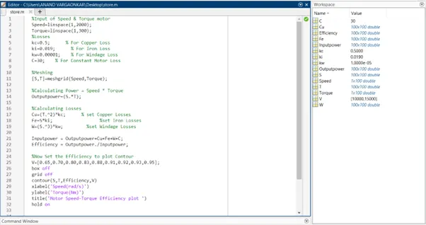
matlab cod -

%Input of Speed & Torque motor
Speed=linspace(1,2000);
Torque=linspace(1,300);
%Losses
kc=0.5;      % For Copper Loss
ki=0.019;      % For Iron Loss
kw=0.00001;    % For Windage Loss
C=30;    % For Constant Motor Loss

%Meshing
[S,T]=meshgrid(Speed,Torque);

%Calculating Power = Speed * Torque
Outputpower=(S.*T);

%Calculating Losses
Cu=(T.^2)*kc;      % set Copper Losses
Fe=S*ki;                  %set Iron Losses
W=(S.^3)*kw;         %set Windage Losses

Inputpower = Outputpower+Cu+Fe+W+C;
Efficiency = Outputpower./Inputpower;

%Now Set the Efficiency to plot Contour
V=[0.65,0.70,0.80,0.83,0.88,0.91,0.92,0.93,0.95];
box off
grid off
contour(S,T,Efficiency,V)
xlabel('Speed(rad/s)')
ylabel('Torque(Nm)')
title('Motor Speed-Torque Efficiency plot ')
hold on


%Additionally Plotting contour 
V=[10000,15000];
contour(S,T,Outputpower,V)

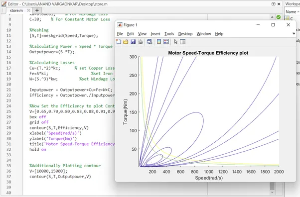
Output –

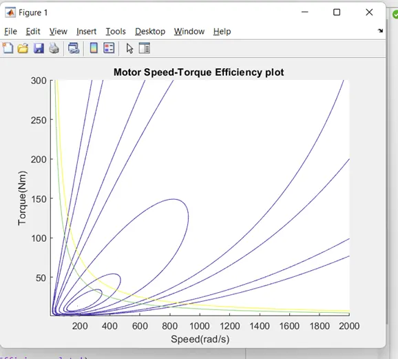
The above Plot shows the Motor Speed-Torque Efficiency Contour Plot. This plot is efficiency is increases in 0.65 to 0.95 %.Increasing efficiency order as going inward and Decreasing efficiency order as going outward. Greater the motor efficiency, lower speed-torque combination is required to overcome the motor losses. this Contour plot clearly gives the idea on Speed, Torque and Efficiency relationship of the motor .