Week-11 Challenge: Braking

1. For a defined driving cycle, calculate the energy required for braking.

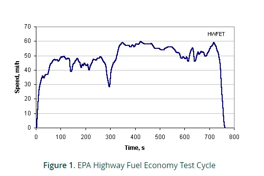
• The Highway Fuel Economy Test (HWFET or HFET) cycle is a chassis dynamometer driving schedule developed by the US EPA for the determination of fuel economy of light duty vehicles is considered for calculation of total braking energy.

The braking energy is given by

Braking Energy = 1/2 * M * (Vf - Vi)^2

where M - Mass of the vehicle, Vi - Initial velocity ; Vf - Final velocity

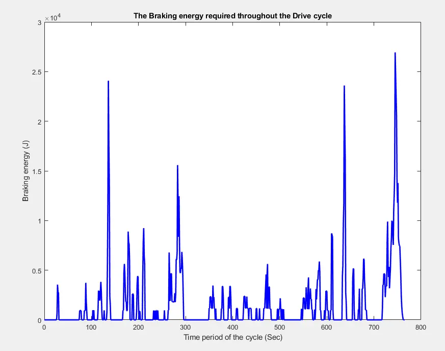
• In the above drive cycle, we can observe deceleration whenever the speed reduces and braking energy is calculated whenever there is a deceleration and summated to get the total braking energy for the drive cycle.
• A mass of 1000 kg is assumed for the vehicle. A matlab code is written to calculate the braking energy.

Matlab code:

clear all
close all
clc
% Mass of the vehicle
M = 1000;
% Total Time period of the cycle
T = 766;
% Read drive cycle data from excel file
A = readmatrix('hwfet.xlsx');
% Time of Drive cycle in seconds
time = A(:,1);
% velocity in mph
velocity = A(:,2);
% convert velocity from mph to m/s 
v = velocity.*0.4470;
% Creating same length vectors for values storage and plotting
Braking_energy=zeros(1,T);

for i = 1:(length(v) - 1)
    if v(i) > v(i+1)

        Braking_energy(i) = 0.5*M*((v(i))^2 - (v(i+1))^2);
        
    end
end

% Plot the Braking energy

plot(time,Braking_energy,'linewidth',2,'color','b')
xlabel('Time period of the cycle (Sec)');
ylabel('Braking energy (J)');
title('The Braking energy required throughout the Drive cycle');

fprintf('The Total Braking Energy Required For HWFET Drive cycle is %3f J',sum(Braking_energy))

Result:

2. Why electric motor can’t develop braking torque at high speed similar to starting? How electric and mechanical brakes are coordinated?

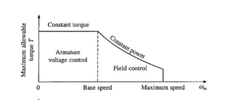
• From the speed-torque curve of a DC motor we can observe the constant torque region where the angular speed of the motor is lower. It is in this phase that the motor is capable to generating the highest torque output. Gradually as the speed increases, the torque decreases which is observed in the constant power region. For this very reason, when the vehicle is operating the high speeds, the angular speed of the motor also will be high and its not possible for the motor to generate a high instantenous braking torque.

Brake Control Strategy -

Mechanical brakes primarily operate on the principle of friction and electric vehicles primarily operate on the principle of engine braking which is otherwise referred to as regenerative braking. However both these types of braking have their own advantages and disadvantages.

Friction braking is very efficient in bringing the vehicle to halt immediately which can be controlled by instantaneously pressing the brake pedal. Most of the energy is dissipated as heat due to friction between the brake pads and discs.

In engine braking, the efficiency of the braking depends on the operating speed of the vehicle. For example, from the above figure we saw that an electric motor can develop high torques at lower speed meaning, at low running speeds, the negative torque can be generated to bring the vehicle to stop almost instantly however in higher speeds, enough braking torque cannot be generated to stop the vehicle immediately. But the advantage here with this kind of braking is that at higher speeds, the kinetic energy of the moving vehicle while decelerating can be used to captured and fed back to charge the battery wherin the motor operates as a generator.

So an electric braking controller will use control strategies based on the vehicle speed data, which type of braking (friction or regenerative) is the best to use depending on its current state of motion. There are various braking modes for different situations the vehicle may face and by utilizing these control strategies, the vehicle can be operating at the highest efficiency at all times and make the best use of the 2 braking mechanisms without damaging or sacrificing one for the other.

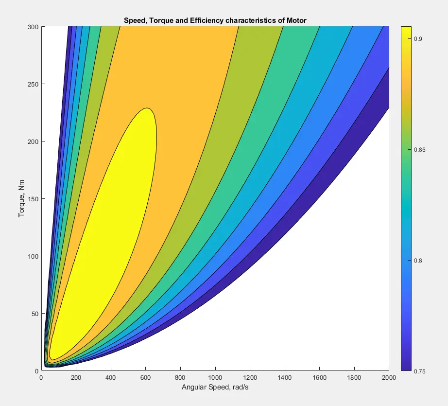
3. Make a MATLAB program which plots contour of given motor speed, torque and efficiency values. Attach the code as a .m file attach a screenshot of all the plots

A contour plot is a 2d plot which visually helps in understanding the characteristics of speed, torque and efficiency for any given motor.

Matlab code:

clear all
close all
clc

% Torque Range
T = linspace(0, 300, 100);
% Speed Range
omega = linspace(0, 2000, 100);
% Meshgrid
[X,Y] = meshgrid(omega, T);
% Loss Coefficients

copper = 0.17;           %Copper losses = `K_(Cu) * omega^2`      
iron = 0.006;            %Iron losses = `K_(Fe) * T^2`           
windage = 0.000015;      %Windage losses = `K_w * T^3`                 

% Losses
copper_loss = copper*(Y.^2);                
iron_loss = iron*(X.^2);             
windage_loss = windage*(X.^3);          
conduction_loss = 18;                    

% Output Power
P_out = (X.*Y);      
% Input Power
P_in = P_out +  (copper_loss) + (iron_loss) + (windage_loss) + (conduction_loss);
% Efficiency
eta = ((P_out)./(P_in));

% Efficiency values for contour
W = linspace(0.75, 0.95, 10);

% Contour Plot

contourf(X,Y,eta,W)
grid off
box off
colorbar
xlabel('Angular Speed, rad/s')
ylabel('Torque, Nm')
zlabel('Efficiency')
title('Speed, Torque and Efficiency characteristics of Motor')

Result: