Week-11 Challenge: Braking

Introduction: The braking performance of a vehicle is undoubtedly one of the important factors to affect vehicle safety. A successfully designed braking system for a vehicle must always meet two distinct demands. Generally, the braking torque required is much larger than the torque that an electric motor can produce. In EVs and HEVs, mechanically frictional braking systems must coexist with electrically regenerative braking.

OBJECTIVES OF THE PROJECT:

For a defined driving cycle, calculate the energy required for braking.

Lets analyze the FTP 75 drive cycle using MATLAB:

%%
%To Calculate the Power Loss in Braking For a Drive Cycle
mass_of_vehicle=1500; %(Kg)
figure(1)
plot(time,v1,'linewidth',2) %plotting the imported drive cycle
xlabel('Time (sec)');
ylabel('Velocity (miles/hr)');
title('FTP 75 Urban Cycle');

%loop to extract braking points in the drive cycle

for i=1:length(time)-1
  
    if Velocity(i) > Velocity(i+1)
        brake_energy(i)=(0.5*mass_of_vehicle*(Velocity(i+1)-Velocity(i))^2)/3600000;  %KWattsHr
    end
        
end
figure(2)
plot(brake_energy,'r');
xlabel('Time (s)');
ylabel('Brake Energy (KWatts-Hr)');
title('FTP 75 Urban Cycle Brake Energy Requirement');
Total_Brake_energy=sum(brake_energy);

Explanation of the Code:

1. First we import the values of Time and velocity as column vectors from the FTP drive cycle data.
2. Then using a if condition we are evaluating when the vehicle deaccelerate and we use these to evaluate the loss in Kinetic energy of the vehicle.
3. This loss is then assigned to the variable brake_energy and using appropriate units we are able to evaluate the loss in K.E for every time step.
4. Using the 'sum(brake_energy)' we evaluate the total energy required for braking.

Lets look at the output plots :

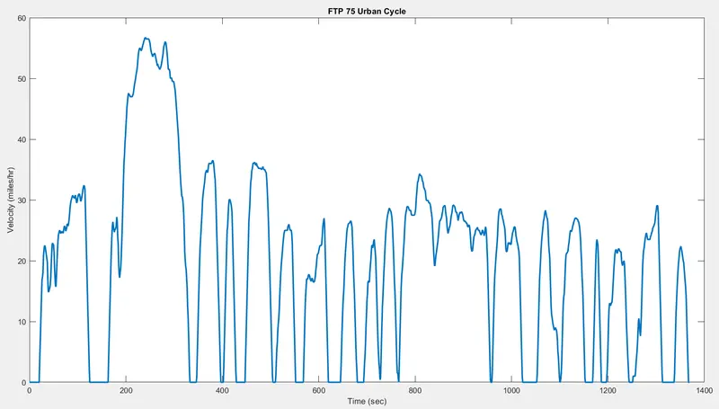
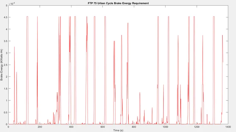
Total energy required for braking is 0.0596 KWatt-Hr.

Why electric motor can’t develop braking torque at high speed similar to starting? How electric and mechanical brakes are coordinated?

It should be noted that the maximum regenerative braking force produced by an electric motor is closely related to the electric motor’s speed. At low speed (lower than its base speed), the maximum torque is constant. However, at high speed (higher than its base speed), the maximum torque decreases hyperbolically with its speed. Therefore, the mechanical brake torque at a given vehicle deceleration varies with vehicle speed.

Generally, the braking torque required is much larger than the torque that an electric motor can produce. In EVs and HEVs, mechanically frictional braking systems must coexist with electrically regenerative braking.

Basically, there are three different brake control strategies: series braking and parallel braking.

Series Braking:

• The braking force on the front wheels (driven axle) is divided into two parts: regenerative braking force and mechanically frictional braking force.
• When the braking force demanded is less than the maximum braking force that the electric motor can produce, only electrically regenerative braking will apply.
• When the commanded braking force is greater than the available regenerative braking force, the electric motor will operate to produce its maximum braking torque, and the remaining braking force is met by the mechanical brake system.

Parallel Braking:

• The parallel brake system includes both an electrical (regenerative) brake and a mechanical brake, which produce braking forces is parallel and simultaneously.
• The parallel brake system has a conventional mechanical brake which has a fixed ratio of braking force distribution on the front and rear wheels.
• Regenerative braking adds additional braking force to the front wheels, resulting in the total braking force distribution curve.

Make a MATLAB program which plots contour of given motor speed, torque and efficiency values. Attach the code as a .m file attach a screenshot of all the plots

% A program for plotting efficiency contours for
% electric motors.
clear all
close all
clc
% First, set up arrays for range.
x=linspace(1,180);% speed,(rad/sec) 
y=linspace(1,40); % 0 to 40 N.m

% Allocate motor loss constants
kc=1.5; % For copper losses
ki=0.1; % For iron losses
kw=0.00001; % For windage losses
Con=20; % For constant motor losses

%Conversion of 1D to 2D array
[X,Y]=meshgrid(x,y);
Output_power=(X.*Y); % Torque x speed = power
B=(Y.^2)*kc; % Copper losses
C=X*ki; % Iron losses
D=(X.^3)*kw; % Windage losses
Input_power = Output_power + B + C + D + Con;
Z = Output_power./Input_power;

% efficiencies for which a contour
% will be plotted.
V=[0.5,0.6,0.7,0.75,0.8,0.85,0.88];

contour(X,Y,Z,V);
xlabel('Speed/rad.s^-^1'),
ylabel('Torque/N.m');

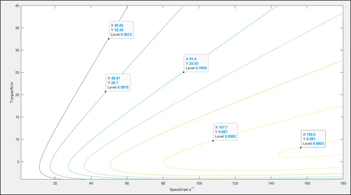
Here in the plot we can identify different efficiency contors, the X represents the speed (rad/sec) and Y represents Torque values in (N-m). Level is representation of the efficiency of the motor.