Week 10 - Simulation of Flow through a pipe in OpenFoam
Poiseuille Flow: It is a pressure induced flow usually in a long duct, a pipe. The flow is assumed to be a laminar flow of an incompressible Newtonian fluid with viscosity µ.
In standard fluid kinetics notation, the pressure drop is represented as
Where Δp = Pressure drop
µ = Dynamic viscosity
L = length of the pipe
Q = volumetric flow of the pipe
R = radius of the pipe
Applications
flow of air in lung alveoli
Flow-through a hypodermic needle
Flow-through a drinking straw
Incompressible flow: In-compressible flow means when the trace of the strain-rate tensor is zero, which means an extension of one coordinate axis is compensated by contraction in another.
Incompressible flow directly manifests that the divergence of the velocity field is zero.
∇ · V =0
Which stands for the derivative of the density is zero. This implies that the fluid density is constant.
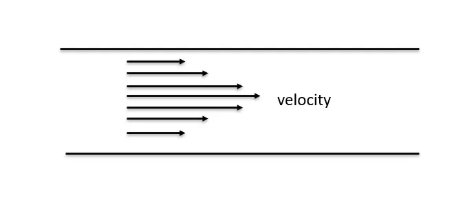
Laminar Flow; it is the property of fluid particles in fluid dynamics to follow smooth paths in layers, with each layer moving smoothly past the adjacent layers with little or no mixing.
From here the parameters of the simulation are calculated using the matlab. Here is the matlab code to create blockmeshdict file.
clear
close all
clc
% Simulation parameters of laminar flow
Re = 2100;
den = 1000;
Dia = 0.02;
Rad = Dia/2;
Length = 0.06*Re*Dia;
mu = 0.00089;
nu = mu/den;
theta = 2;
% Defining the Boundary condition
v_avg = Re*nu/Dia;
v_max = 2*v_avg;
l = Length + 0.3;
deltap = (8*v_avg*mu*l)/Rad^2;
% Vertices and coordinates in the local coordinate system
v0 = [0 0 0];
v1 = [0 Rad*cosd(theta/2) -Rad*sind(theta/2)];
v2 = [0 Rad*cosd(theta/2) Rad*sind(theta/2)];
v3 = [Length 0 0];
v4 = [Length Rad*cosd(theta/2) -Rad*sind(theta/2)];
v5 = [Length Rad*cosd(theta/2) Rad*sind(theta/2)];
grading = 0.2;
b1 = 50;
b2 = 1;
b3 = 200;
% Creating BlockMesh file code for OpenFOAM in its official format
% The first section of OpenFOAM description
h1 = '/*--------------------------------*- C++ -*----------------------------------*\';
h2 = '| ========= | |';
h3 = '| \\ / F ield | OpenFOAM: The Open Source CFD Toolbox |';
h4 = '| \\ / O peration | Website: https://openfoam.org |';
h5 = '| \\ / A nd | Version: 11 |';
h6 = '| \\ / M anipulation | |';
h7 = '\*---------------------------------------------------------------------------*/';
% Writing and creating the BlockMesh file which is writable
f1 = fopen('blockMeshDict.txt', 'wt');
fprintf(f1, '%s\n', h1);
fprintf(f1, '%s\n', h2);
fprintf(f1, '%s\n', h3);
fprintf(f1, '%s\n', h4);
fprintf(f1, '%s\n', h5);
fprintf(f1, '%s\n\n', h6);
fprintf(f1, '%s\n\n', h7);
% Second section of the file where the parameters are initialized and simulated with time steps
fprintf(f1, 'FoamFile\n{\n');
fprintf(f1, '%16s %10s\n', 'version', '2.0;');
fprintf(f1, '%16s %12s\n', 'format', 'ascii;');
fprintf(f1, '%16s %17s\n', 'class', 'dictionary;');
fprintf(f1, '%16s %20s\n', 'object', 'blockMeshDict;');
fprintf(f1, '}\n\n');
% The third section of the parameters
fprintf(f1, '%s\n\n', '// * * * * * * * * * * * * * * * * * * * * * * * * * * * * * * * * * * * * * //');
fprintf(f1, 'convertToMeters 1;\n');
fprintf(f1, 'vertices\n(\n');
fprintf(f1, ' (%f %f %f)\n', v0);
fprintf(f1, ' (%f %f %f)\n', v1);
fprintf(f1, ' (%f %f %f)\n', v2);
fprintf(f1, ' (%f %f %f)\n', v3);
fprintf(f1, ' (%f %f %f)\n', v4);
fprintf(f1, ' (%f %f %f)\n', v5);
fprintf(f1, ');\n\n');
% Defining the flow parameters in the file
fprintf(f1, 'blocks\n(\n');
fprintf(f1, ' hex (0 1 2 0 3 4 5 3) (%d %d %d) simpleGrading (%f 1 1)\n', b1, b2, b3, grading);
fprintf(f1, ');\n\n');
fprintf(f1, 'edges\n(\n');
fprintf(f1, ' arc 1 2 (0 %f 0)\n', Rad);
fprintf(f1, ' arc 4 5 (%f %f 0)\n', Length, Rad);
fprintf(f1, ');\n\n');
fprintf(f1, 'boundary\n(\n');
fprintf(f1, ' axis\n {\n');
fprintf(f1, ' type empty;\n');
fprintf(f1, ' faces\n (\n');
fprintf(f1, ' (0 3 3 0)\n');
fprintf(f1, ' );\n');
fprintf(f1, ' }\n');
fprintf(f1, ' wall\n {\n');
fprintf(f1, ' type wall;\n');
fprintf(f1, ' faces\n (\n');
fprintf(f1, ' (2 5 4 1)\n');
fprintf(f1, ' );\n');
fprintf(f1, ' }\n');
fprintf(f1, ' inlet\n {\n');
fprintf(f1, ' type patch;\n');
fprintf(f1, ' faces\n (\n');
fprintf(f1, ' (0 0 2 1)\n');
fprintf(f1, ' );\n');
fprintf(f1, ' }\n');
fprintf(f1, ' outlet\n {\n');
fprintf(f1, ' type patch;\n');
fprintf(f1, ' faces\n (\n');
fprintf(f1, ' (3 4 5 3)\n');
fprintf(f1, ' );\n');
fprintf(f1, ' }\n');
fprintf(f1, ' wedgeFront\n {\n');
fprintf(f1, ' type wedge;\n');
fprintf(f1, ' faces\n (\n');
fprintf(f1, ' (0 3 5 2)\n');
fprintf(f1, ' );\n');
fprintf(f1, ' }\n');
fprintf(f1, ' wedgeBack\n {\n');
fprintf(f1, ' type wedge;\n');
fprintf(f1, ' faces\n (\n');
fprintf(f1, ' (0 1 4 3)\n');
fprintf(f1, ' );\n');
fprintf(f1, ' }\n');
fprintf(f1, ');\n\n');
fprintf(f1, 'mergePatchPairs\n(\n);\n\n');
fprintf(f1, '%s\n', '// * * * * * * * * * * * * * * * * * * * * * * * * * * * * * * * * * * * * * //');
% Finally closing the file
fclose(f1);
After running this code we will get blockMeshdict file which will be transferred to solver that we are working on.we will be using the icoFoam solver for the simulation. The following are the input and boundary condition files.
blockMeshDict File:
/*--------------------------------*- C++ -*----------------------------------*\ | ========= | | | \\ / F ield | OpenFOAM: The Open Source CFD Toolbox | | \\ / O peration | Website: https://openfoam.org | | \\ / A nd | Version: 11 | | \\ / M anipulation | | \*---------------------------------------------------------------------------*/ FoamFile { version 2.0; format ascii; class dictionary; object blockMeshDict; } // * * * * * * * * * * * * * * * * * * * * * * * * * * * * * * * * * * * * * // convertToMeters 1; vertices ( (0.000000 0.000000 0.000000) (0.000000 0.009998 -0.000175) (0.000000 0.009998 0.000175) (2.520000 0.000000 0.000000) (2.520000 0.009998 -0.000175) (2.520000 0.009998 0.000175) ); blocks ( hex (0 1 2 0 3 4 5 3) (50 1 200) simpleGrading (0.200000 1 1) ); edges ( arc 1 2 (0 0.010000 0) arc 4 5 (2.520000 0.010000 0) ); boundary ( axis { type empty; faces ( (0 3 3 0) ); } wall { type wall; faces ( (2 5 4 1) ); } inlet { type patch; faces ( (0 0 2 1) ); } outlet { type patch; faces ( (3 4 5 3) ); } wedgeFront { type wedge; faces ( (0 3 5 2) ); } wedgeBack { type wedge; faces ( (0 1 4 3) ); } ); mergePatchPairs ( ); // * * * * * * * * * * * * * * * * * * * * * * * * * * * * * * * * * * * * * //
ControlDict File:
*--------------------------------*- C++ -*----------------------------------*\
| ========= | |
| \\ / F ield | OpenFOAM: The Open Source CFD Toolbox |
| \\ / O peration | Version: v2312 |
| \\ / A nd | Website: www.openfoam.com |
| \\/ M anipulation | |
\*---------------------------------------------------------------------------*/
FoamFile
{
version 2.0;
format ascii;
class dictionary;
object controlDict;
}
// * * * * * * * * * * * * * * * * * * * * * * * * * * * * * * * * * * * * * //
application icoFoam;
startFrom startTime;
startTime 0;
stopAt endTime;
endTime 10;
deltaT 0.005;
writeControl timeStep;
writeInterval 20;
purgeWrite 0;
writeFormat ascii;
writePrecision 6;
writeCompression off;
timeFormat general;
timePrecision 6;
runTimeModifiable true;
// ************************************************************************* //
Transport Properties:
*--------------------------------*- C++ -*----------------------------------*\
| ========= | |
| \\ / F ield | OpenFOAM: The Open Source CFD Toolbox |
| \\ / O peration | Version: v2312 |
| \\ / A nd | Website: www.openfoam.com |
| \\/ M anipulation | |
\*---------------------------------------------------------------------------*/
FoamFile
{
version 2.0;
format ascii;
class dictionary;
object transportProperties;
}
// * * * * * * * * * * * * * * * * * * * * * * * * * * * * * * * * * * * * * //
nu [0 2 -1 0 0 0 0] 8.9e-07;
// ************************************************************************* //
Here are the conditions of velocity and pressure for the flow.
VELOCITY
/*--------------------------------*- C++ -*----------------------------------*\
| ========= | |
| \\ / F ield | OpenFOAM: The Open Source CFD Toolbox |
| \\ / O peration | Version: v2312 |
| \\ / A nd | Website: www.openfoam.com |
| \\/ M anipulation | |
\*---------------------------------------------------------------------------*/
FoamFile
{
version 2.0;
format ascii;
class volVectorField;
object U;
}
// * * * * * * * * * * * * * * * * * * * * * * * * * * * * * * * * * * * * * //
dimensions [0 1 -1 0 0 0 0];
internalField uniform (0 0 0);
boundaryField
{
inlet
{
type fixedValue;
value uniform (0.1869 0 0);
}
outlet
{
type zeroGradient;
}
wedgeFront
{
type wedge;
}
wedgeBack
{
type wedge;
}
wall
{
type noSlip;
}
axis
{
type empty;
}
}
// ************************************************************************* //
PRESSURE:
/*--------------------------------*- C++ -*----------------------------------*\
| ========= | |
| \\ / F ield | OpenFOAM: The Open Source CFD Toolbox |
| \\ / O peration | Version: v2312 |
| \\ / A nd | Website: www.openfoam.com |
| \\/ M anipulation | |
\*---------------------------------------------------------------------------*/
FoamFile
{
version 2.0;
format ascii;
class volScalarField;
object p;
}
// * * * * * * * * * * * * * * * * * * * * * * * * * * * * * * * * * * * * * //
dimensions [0 2 -2 0 0 0 0];
internalField uniform 0;
boundaryField
{
inlet
{
type zeroGradient;
}
outlet
{
type fixedValue;
value uniform 0;
}
wall
{
type zeroGradient;
}
// top
// {
// type zeroGradient;
// }
axis
{
type empty;
}
wedgeFront
{
type wedge;
}
wedgeBack
{
type wedge;
}
}
// ************************************************************************* //
velocity from openfoam and analytical values are compared here.The code for analytical velocity profile is attached below.
% Parameters
pipeDiameter = 0.02; % Example diameter
numPoints = 100;
maxVelocity = 0.1869; % Example max velocity
[u_analytical, r] = analyticalVelocityProfile(pipeDiameter, numPoints, maxVelocity);
figure;
plot(r, u_analytical, 'g-', 'LineWidth', 2);
xlabel('x Position (m)');
ylabel('Velocity (m/s)');
title('Velocity Profile');
legend('Analytical');
grid on
% Analytical velocity profile for Hagen-Poiseuille flow
function [u_analytical, r] = analyticalVelocityProfile(pipeDiameter, numPoints, maxVelocity)
r = linspace(0, pipeDiameter/2, numPoints);
u_analytical = maxVelocity * (1 - (2*r/pipeDiameter).^2);
end
Graphs from openfoam and analytical:
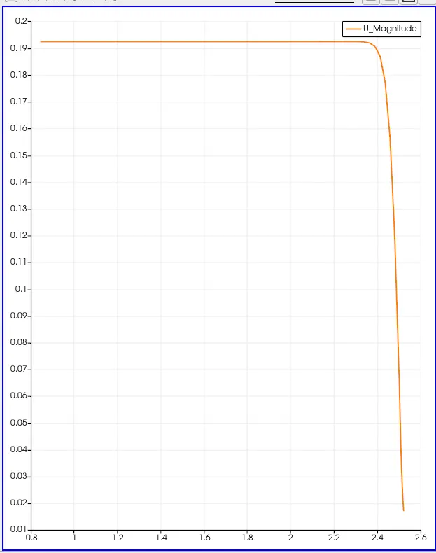
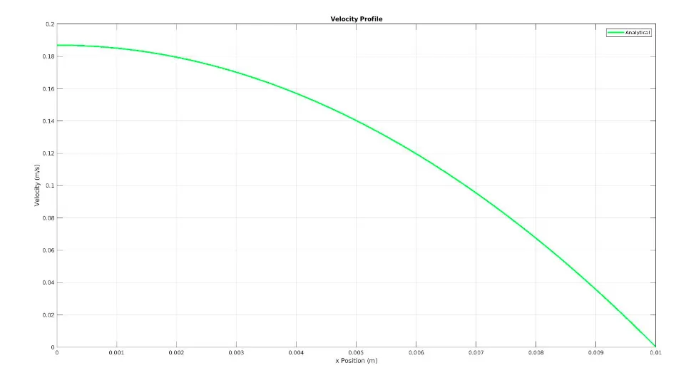
Conclusion for velocity profile:
The velocity profile from both the analytical and OpenFOAM numerical simulations agrees quite well. Observations show that the velocity profile increases gradually along the length of the pipe, reaching its maximum at the outlet. This region, known as the fully developed region, is where the velocity profile fully develops at the outlet.
As the fluid flows, shear stresses develop due to the relative motion of the particles within the flow. In a pipe, the fluid velocity is zero at the pipe wall due to no-slip boundary conditions. Shear force arises because adjacent fluid layers move at different velocities. At the walls, the velocity remains zero, while as the flow progresses, boundary layers develop and adjacent layers slow down. Consequently, the velocity at the center increases. Therefore, due to the pressure difference obtained from the equations, the velocity profile follows Hagen-Poiseuille's equation, matching the analytical solution.
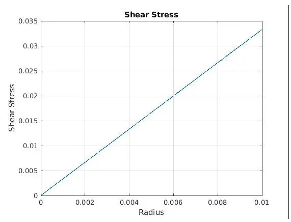
Pressure drop and shear stress plots:
Wall shear stress expresses the retarding force from a wall in the layers of a fluid flowing next to the wall. It is defined as:
Tau=  *d
*d /dy
/dy
where is the dynamic viscosity, the flow velocity and  the distance from the wall.
here are the pressure profile and shear stress plots from the openfoam and matlab codes.
Pressure profile.
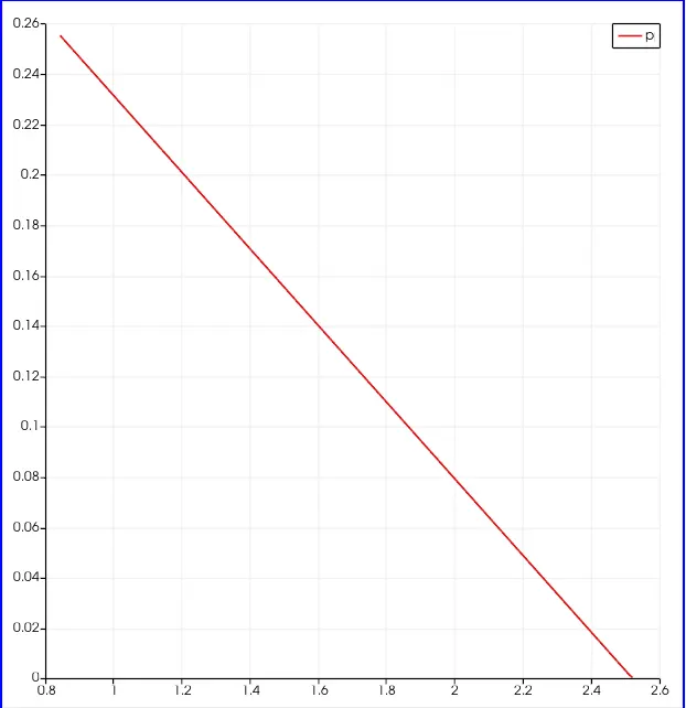
If we calculate the pressure drop from this graph at any location using pressure from the graph and other fluid properties the values does match.
As per the shear stress profile the following code is used to get the graph
clear
close all
clc
% Parameters
Re=2100;
Dia= 0.02;
Rad=Dia/2;
kin_v=0.00089;
den=1000;
kin_v=kin_v/den;
%analytical calculation
L_e=0.06*Re*Dia;
L_t=L_e+0.3;
avg_vel=(Re*kin_v)/Dia;
max_vel=2*avg_vel;
Delta_P=(8*kin_v*avg_vel*L_t)/Rad^2;
kin_P=Delta_P/den;
j= linspace(0,Rad,1000);
for i=1:length(j)
ss(i)=2*kin_v*max_vel*(abs(j(i)))/Rad^2;
end
figure(1)
plot(j,ss)
grid on
hold on
title("Shear Stress")
xlabel("Radius")
ylabel('Shear Stress')
All of the commands used for the simulation are attached in txt file.
References:
1.https://en.wikipedia.org/wiki/Hagen%E2%80%93Poiseuille_equation
2.https://www.youtube.com/watch?v=R3sa9_O938A
3.https://en.wikipedia.org/wiki/Shear_stress