Week 10 - Simulating Combustion of Natural Gas.

Combustion Simulation

Aim:-

To simulate a two dimensional combustion simulation for investigating the concentration of Soot and Pollutant formation during reaction. The first test case consist of fuel as methane and air combustion and then we analysis the formation of soot and pollutant particle formed. In second test case we add water with the fuel and analysis the reduction in soot and pollutant formation.

Introduction:-

The emission of the particle matter, soot can be consider as a side effect associate to combustion process characterised by high temperature and rich condition. The production of these nanoparticle entails a reduction in the efficiency of the combustion device, as well as detrimental effect on climate change and human health. Therefore, a drastic reduction in emissions is mandatory, demanding for a deeper understanding in the formation process, which is still an open issue in combustion chemistry research. In the past years strategies for the reduction in soot emissions relied mainly on correlations, experience and trial-and-error attempts. The increasingly diffusion of CFD is allowing to analyze and optimize combustion devices with sufficient confidence. However, the uncertainty increases significantly when soot is concerned: the complexity of the gas-phase chemistry and the numerous mechanisms involved in soot formation process, which are strongly coupled with mixing and radiative heat transfer and depend on soot volume fraction itself, make the prediction of soot emissions still a challenging task, leading to large errors in exhaust concentration even with small mispredictions in the formation rates . Different mechanisms are in fact involved in the determination of the final concentration at the exit of the combustion device, such as inception, coagulation, surface growth and oxidation. Even though reasonable predictions can be achieved on laminar diffusion flames , the scenario is further complicated when turbulent flames burning common fuels such as diesel or kerosene are concerned, as the applicability of models developed for simple aliphatic hydrocarbon fuels (such as methane) is questioned. Soot production in methane-air flames usually takes place from small species (e.g. acetylene) that grow to form polyaromatic hydrocarbons (PAH) and eventually soot. However, practical fuels such as kerosene contains aromatics, which significantly accelerate the soot formation process.

Theory:-

Soot models can be classified on the basis of their complexity and computational effort involved. According to Kennedy , a distinction can be made in three categories: empirical, semi-empirical and detailed models. One of the most known empirical model was proposed by Khan et al. to predict soot emissions in diesel engines and, neglecting particle growth and oxidation rates, estimates soot formation as a function of pressure, temperature and equivalence ratio of unburnt gases. A more accurate description of the physics can be obtained with semi-empirical models that include the chemical processes involved in soot formation, for example, expressing particle inception and surface growth on the basis of PAH concentration. Lindstedt et al. exploited simplified reactions to describe the formation and growth of soot particles in laminar non-premixed ethylene and propane flames, using benzene and acetylene as precursors. Other example are given by Fairweather et al. and Brookes and Moss, which differ for the choice of the precursor to soot nucleation, the model constants or the oxidation mechanism. High-fidelity predictions in a wider range of fuels and operating conditions require to account for the dependency of soot inception and surface growth on the PAH concentration. Detailed chemistry mechanisms are required to estimate PAH formation, whereas additional pathways should be considered for surface reactions, as well as the agglomeration of soot particles in complex agglomerate structures. This is accomplished with Monte Carlo models, sectional methods or methods of moments (refer to Mueller et al. for a description of these techniques). After this overview, the soot models investigated in the present work are presented here below.

Pre-processing and meshing:-

A predefined geometry is imported to ANSYS Spacecliam .the geometry contains a three cylinder as shown in Figure 1 for our present analysis we are interested to take a 2D geometry because its robust and simplified. Therefore first we split the 3D model in to two half by using split body command Split body command. After splitting all three cylinder to two half we hide one haft section and then copy the surface and paste it to new file. The new surface is generated buy it contains a three section so we have to combine it to one surface, this is done by using the combine tool as shown in Figure 2. After geometry is completed we further move toward the meshing section.

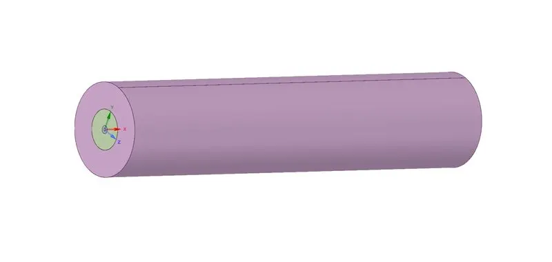
Figure 1, importd geometry. Figure 2, extracted surface

In the following meshing section we do a size control of 1.5 mm. to refine a mesh under the area where the fuel is entered we check the capture proximity option and apply a number of cell across gap to 3. Multizone method is selected with all quad elements. A Figure 3 shown the meshed surface. with this mesh quality we can get a number of node 32302 and number of element 31653. A Figure 4 and 5 shows the name selection given to walls.

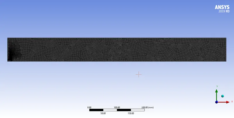
Figure 3, meshed surface

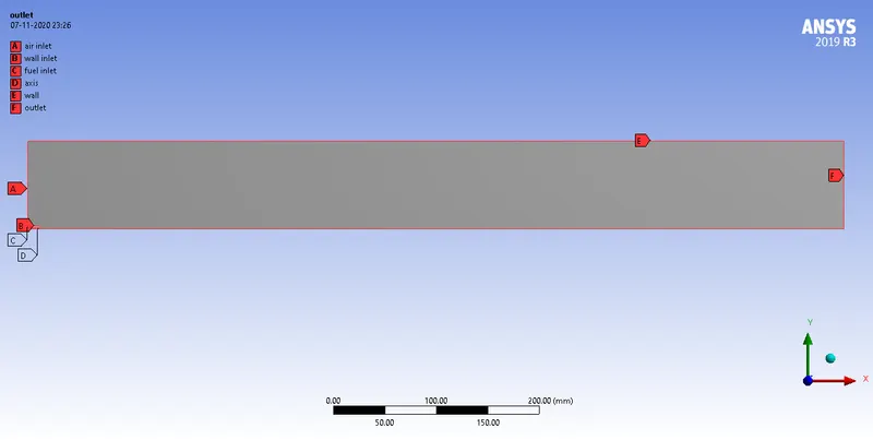
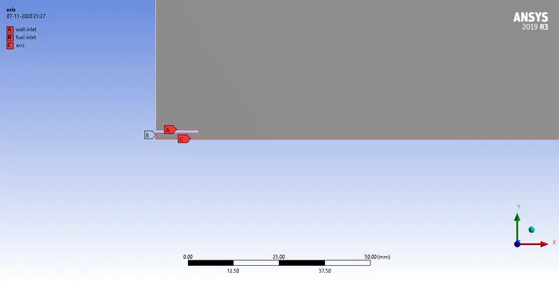
Figure 4, geometry named selection. Figure 5, geometry named selection.

Solver setup:-

For our first test case ,based on the above mesh , here we choose a pressure based solver with 2D axisymmetric option. For turbulence modelling we chose a Standard K-e turbulence model with standard wall function. Energy equations are on. Now for species transport window we have to activate a Specious transport model with reaction to volumetric with inlet diffusion and diffusion energy source option checked. In mixture property we choose a methane-air material. Turbulence chemistry interaction to Eddy dissipation. After that under specious transport bar we have to on NOx model for calculating the pollutant concentration. In NOx model window under formation -pathway we have to check thermal NOx And promt NOx. In fuel species we have to select methane. Now for calculating the soot formation we have to activate the soot one step model.

For boundary condition the air inlet is selected as velocity inlet with air velocity as 0.5 m/s and hydraulic diameter as 0.0826 m, under the species option the mas fraction of oxygen is 0.23. for fuel inlet we choose a velocity inlet with magnitude of 80 m/s. and hydraulic diameter as 0.001652 m , under species tab the mass fraction of methane should be 1. Axis is selected as axis and wall as wall. Pressure velocity coupling scheme as Coupled. Then we initialized the solution by using he hybrid initialization. And run the calculation for 600 iteration.

For our second test case we have to add water with the fuel for that e have to add mixture material as methane air two step under species model tab. under NOx model we have to add both methane and water as a fuel species. After that we have to change the mole fraction of fuel and water entering through the fuel inlet we put mole fraction of methane as 0.75 and mole fraction of water as 0.25. Everything else remains the same .now in this case we are going to add water with fuel and increase its quantity and investigate the amount of soot formation and pollutant with increase in water quantity. initialised the solution by using hybrid initialisation and run the calculation for 600 iteration.

Result:-

The analysed result for first case showing different chemical compounds involved in reaction which are CH4,H2O,CO2,N2,O2 pollutant NO and Soot. To study the behaviour of various compound along the length of the chamber we have created 13 vertical line places at equal distance from inlet to outlet inside the combustion chamber. Figure 6 shows the contour image of CH4 formation during the combustion. We can see that the mass fraction of methane is high at the fuel inlet. As combustion start the mass fraction is going to reduce along the length. In Figure 7 shows the plot of CH4 on all 13 lines. Here we can see that for the point near to axis line and inlet have a high amount of methane. But along the length of line at top of the wall the mass fraction is very low. Also as we move toward the outlet the mass fraction of methane is decreased in steady manner from line 1 to 8 the mass fraction is high at the axis and the from line 9 to 13 its concentrations is remain constant and low . For CO2 the contour plot shown in Figure 8 . the mass fraction is high at the axis line and propagate along the length of chamber up to mid and then reduced at the outlet. Figure 9 shows the plot of mass fraction of CO2 here we see that on the vertical line we have high value near he axis but as go to up near the wall the value is very low. Also the values for line 1 to 6 show an unstable behaviour but for line 7 to 13 the value is nearly constant and shows a low deflection . so we can say that the outlet value is nearly equal to 0.1. for H2O it also shows the same behaviour a that of CO2 as show in Figure 10 and 11. For N2 , mass fraction is very high above the fuel inlet , mass fraction is very low near the fuel inlet. But then the value is high at 0.75 in overall chamber as shown in Figure 12. The line plot shown in Figure 13 shows that mass faction remains constant in over all chamber.

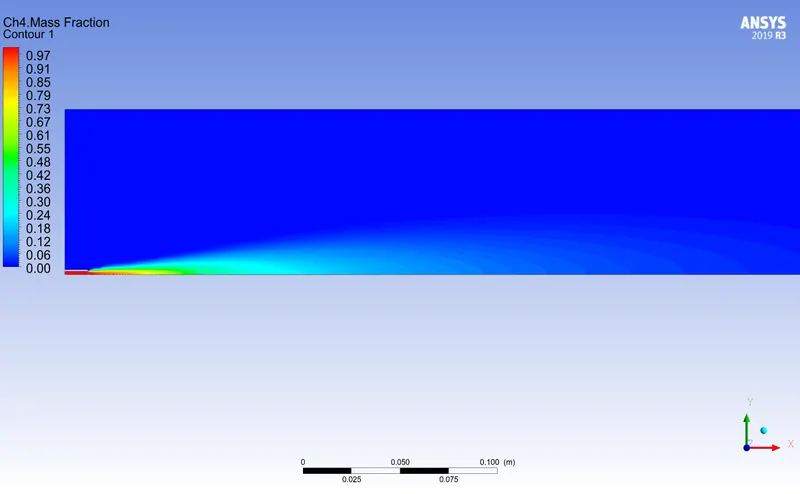
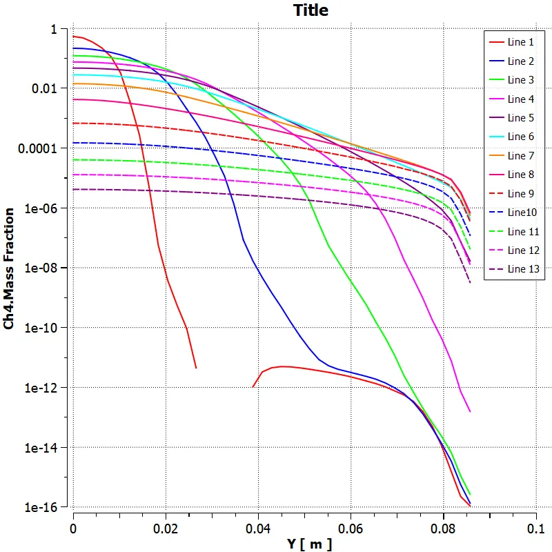
Figure 6, Contour pot of CH4 mass fraction. Figure 7, Line plot of CH4 mass fraction

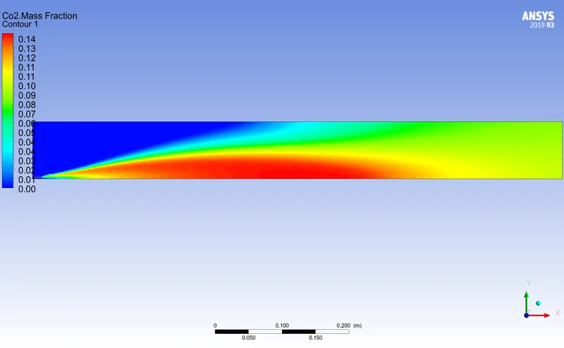
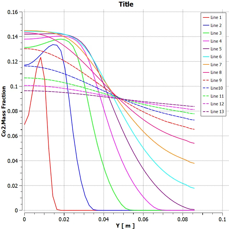
Figure 8, Contour plot of CO2 mass fration. Figure 9, Line plot of CO2 mass fraction.

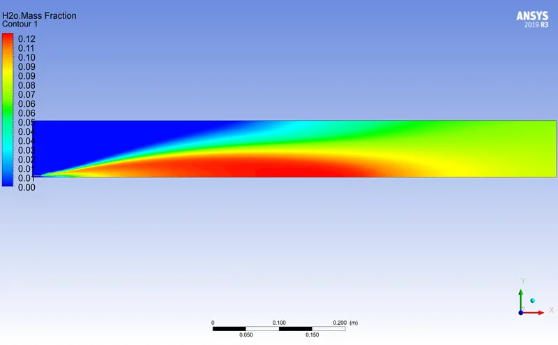
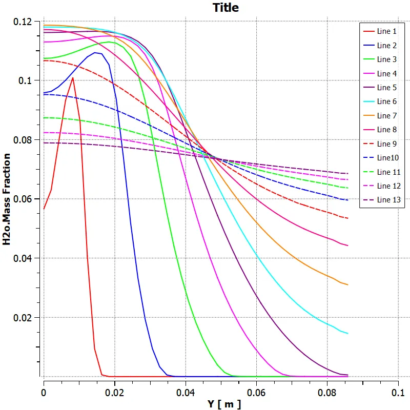
Figure 10, Contour plot of mass fravtion of H2O. Figure 11, Line plot of mass fraction of H2O.

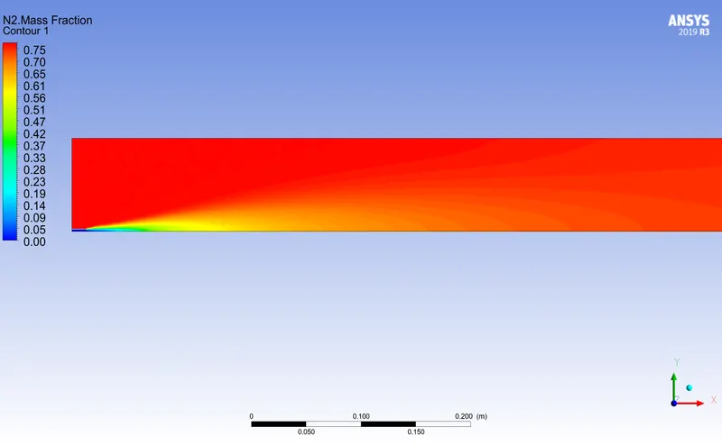
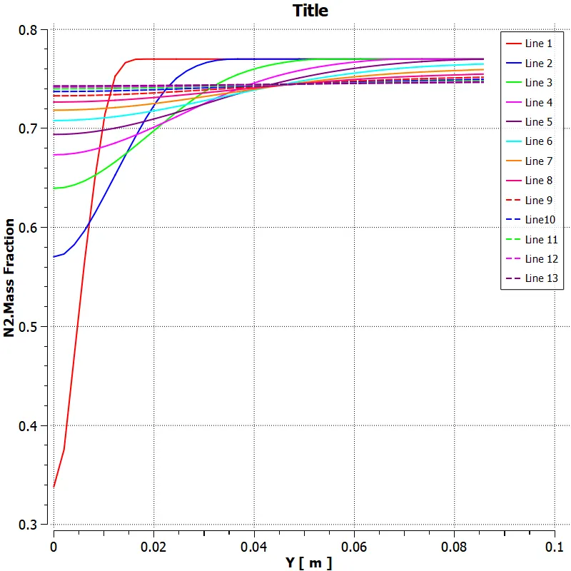
Figure 12, Contour plot of mass fravtion of N2. Figure 13, Line plot of mass fraction of N2.

For pollutant NO we can see that mass fraction is high after themed section and at the outlet as shown in Figure 14. Also from the line plot we can see that for a line from 8 to 13 the mass fraction of pollutant is high . also the value is low at the top wall portion as shown in Figure 15. Now for O2 from the Figure 16 we can say that its concentration is high at upper portion near the wall and low at the axis. So when combustions start oxygen is consumed at that area and them its mass fraction value seem to constant from line 7 to 13 as shown in Figure 17. From the result we can see the soot formation after combustion as shown in Figure 18 and Figure 19 and it value is 1e-36 at the outlet. At last the temperature profile is shown in Figure 20, from that we can say at after the combustion is started the temperature is high up the mid of chamber and then its value is decreased at the outlet.

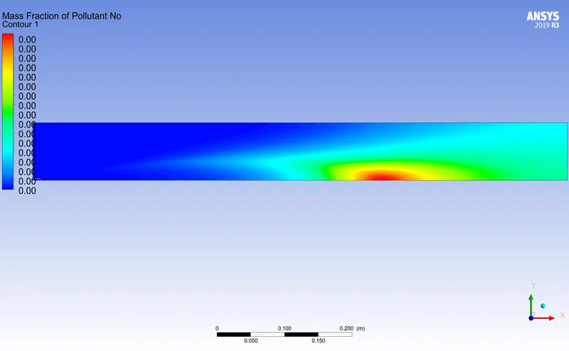
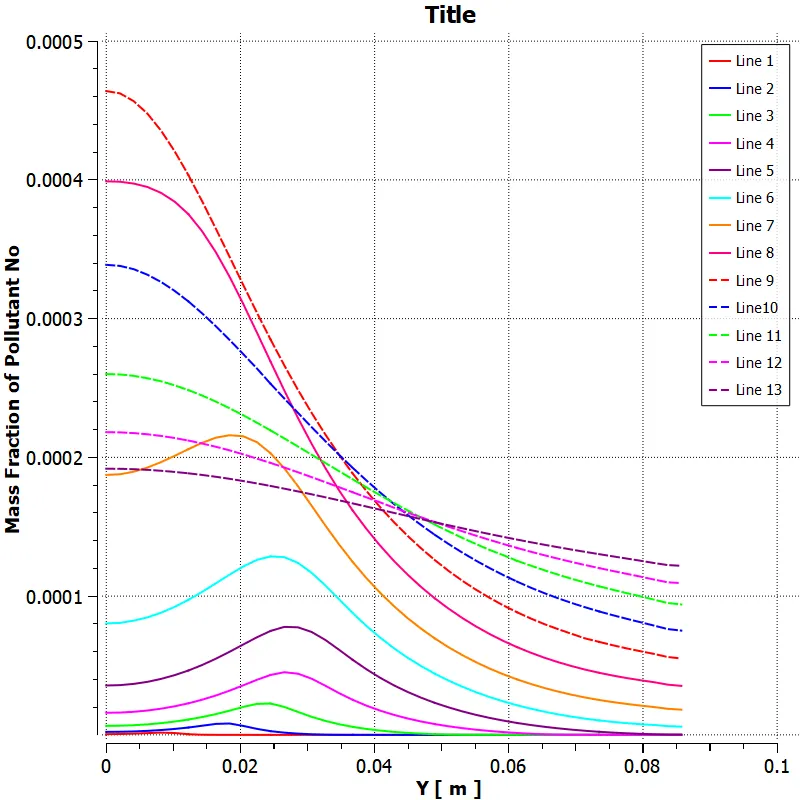
Figure 14, Contour plot of mass fraction for pollutant NO. Figure 15, Line plot of mass fraction of pollutant NO.

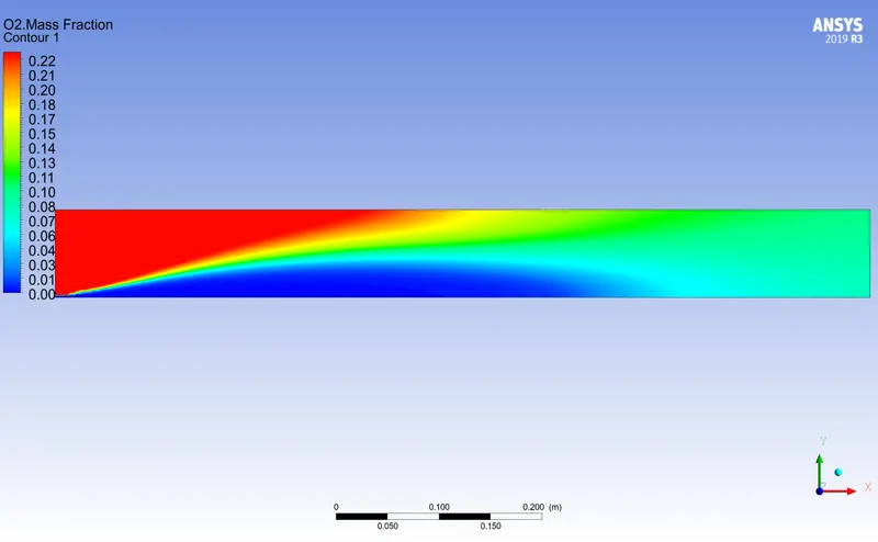
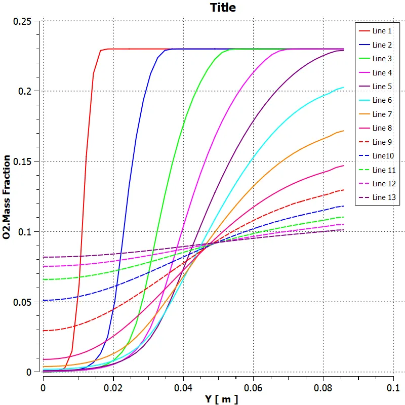
Figure 16, Contour plot of mass fraction for pollutant O2. Figure 17, Line plot of mass fraction of pollutant O2.

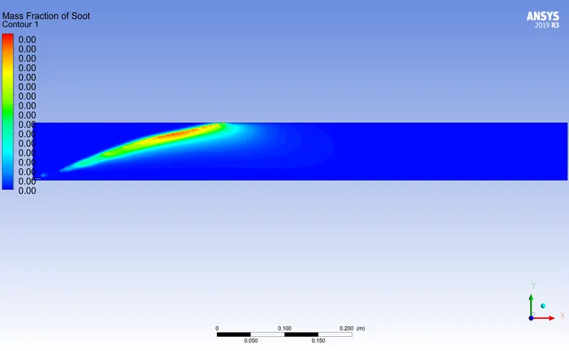
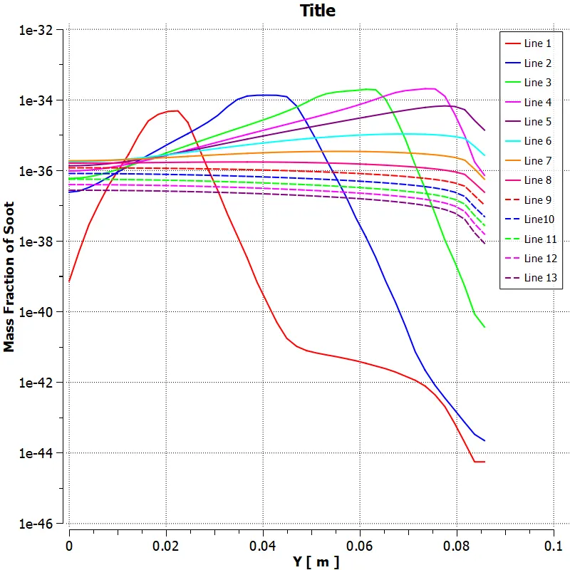
Figure 18, Contour plot of mass fraction for Soot particle. Figure 19, Line plot of mass fraction for Soot particle.

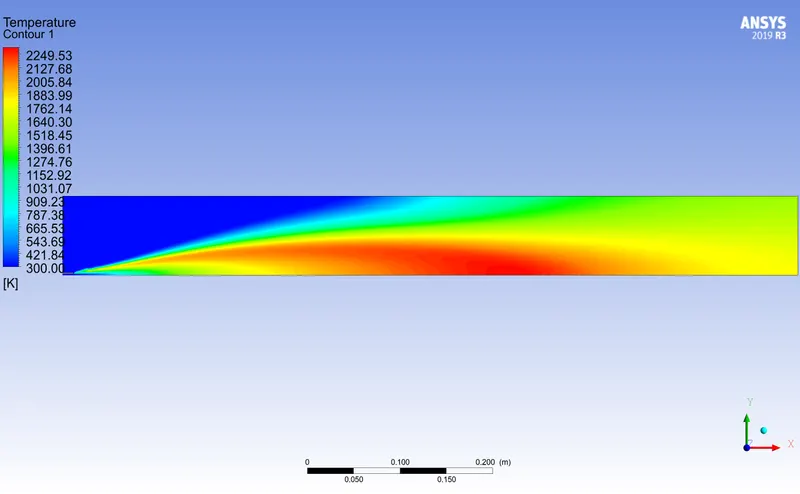
Figure 20, Temperature contour of combustion chamber.

For our second test case we are adding water with fuel and increasing its concentration. So we adding water in fuel with varying its concentration from 5% to 30%. Now for CH4 we can see that as the water concentration is increased in from the methane concentration at outlet is reduced as shown in Figure 21. We can see the same for the CO ,H2O and CO2 shown in Figure 22 ,23 and 24. In case of N2 we can see that at outlet near the axis its concentration is low and at the top wall is high also the N2 , concentration is increasing as we add water concentration in fuel as show in Figure 25. Mass fraction of O2 is also increasing as we water concentration is increased in fuel as shown in Figure 26 . Now for most important matter the pollutant NO and soot , we can see that both are decreased with increased in water in fuel as shown in Figure 27 and 28.

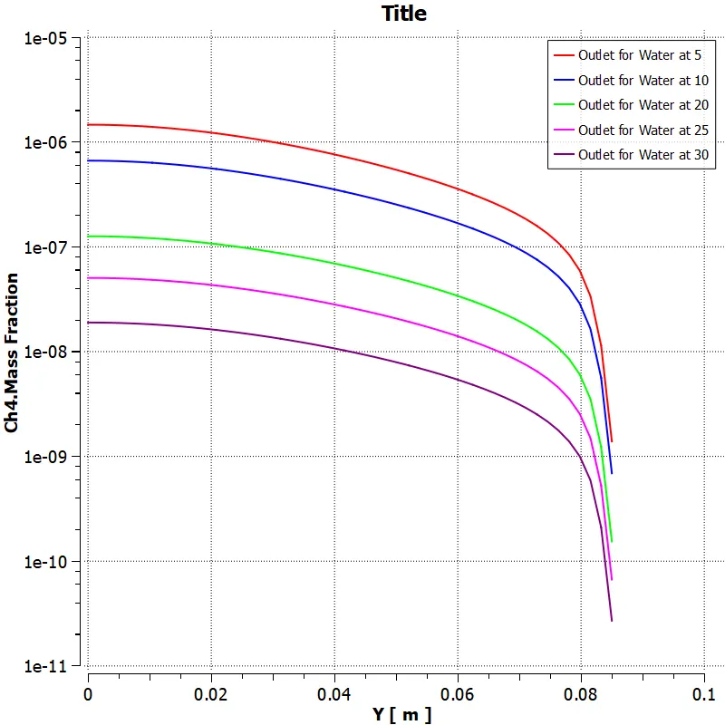
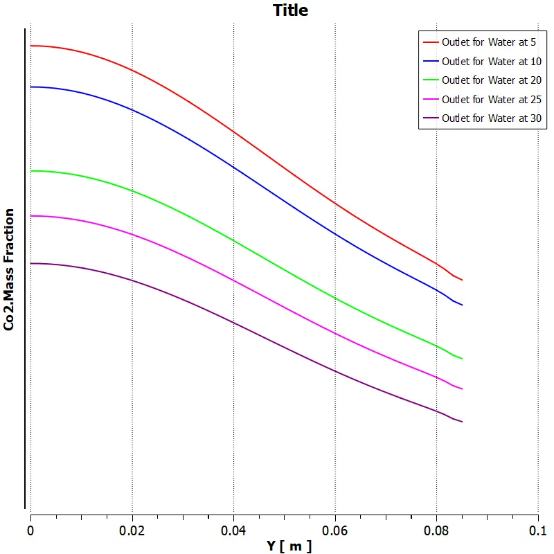
Figure 21, Mass fraction of CH4,at different water concentration. Figure 22, Mass fraction of CO2,at different water concentration.

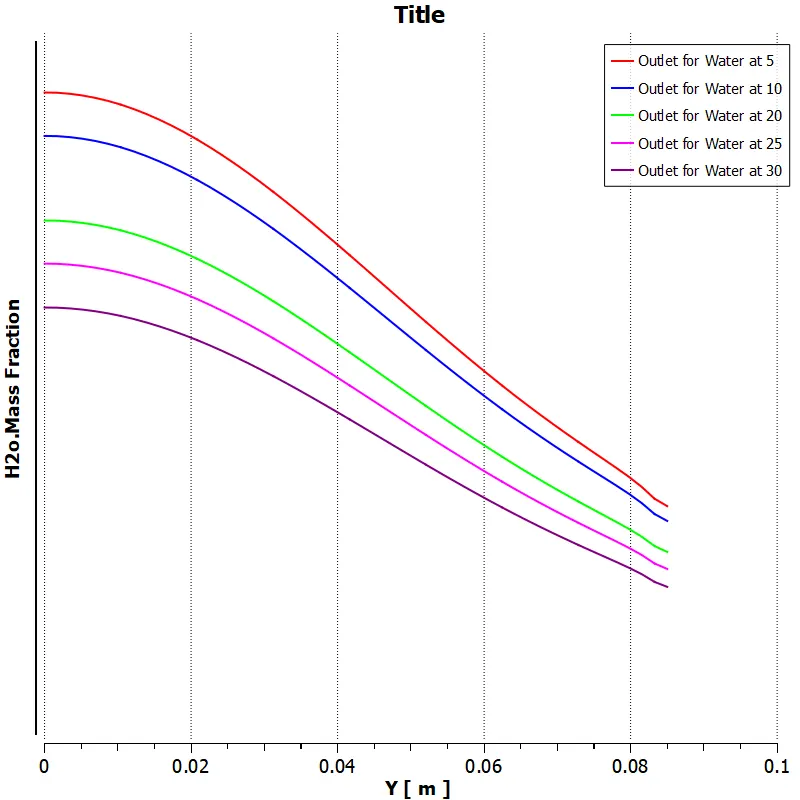
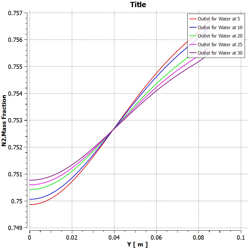
Figure 23, Mass fraction of H2O,at different water concentration. Figure 24, Mass fraction of N2,at different water concentration.

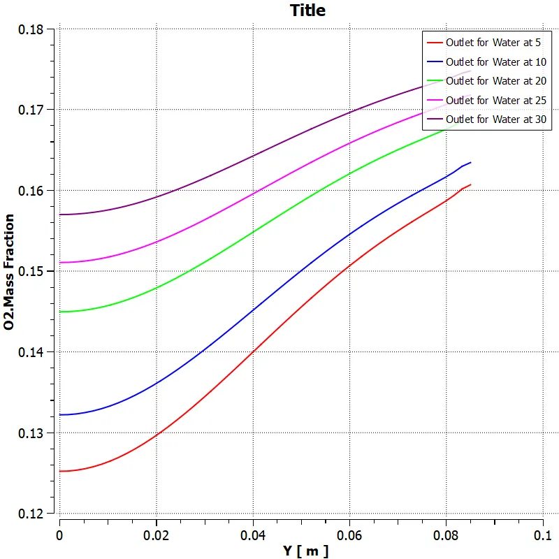
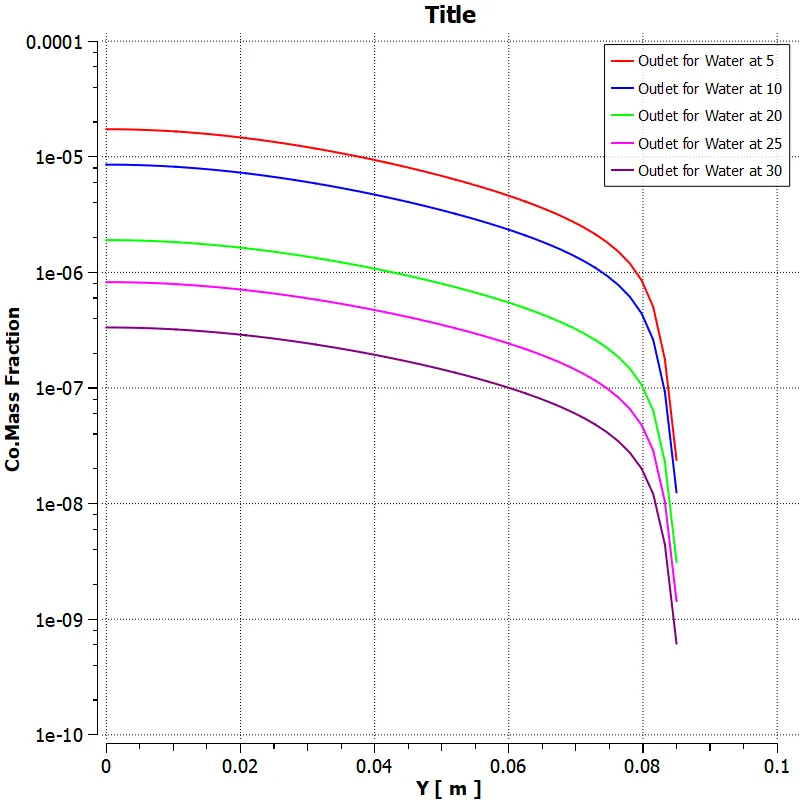
Figure 25, Mass fraction of O2,at different water concentration. Figure 26, Mass fraction of CO,at different water concentration.

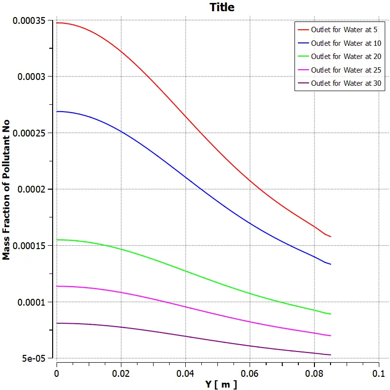
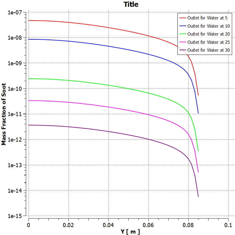
Figure 21, Mass fraction of NO,at different water concentration. Figure 21, Mass fraction of Soot,at different water concentration.

Conclusion:-

A two dimensional combustion simulation is performed on a chamber with a mixture fuel as a methane. Two test case is carried to analyse the combustion . for the first test case e are looked how concentration of all reactant in the combustion is varied. So from the simulation we can say that CH4 mass fraction is only high area near to the fuel inlet and for CO2 its concentration is high on the axis region and low at the outlet , water behaves in the same . but for the N2 its concentration is high for the entire region except near to the combustion area. O2 mass fraction is also low at the outlet but we can see a smooth transaction from the combustion region to upper region. For the pollutant NO an the soot their mass fraction is high at the outlet.

Now for our second test case we see that as we add water to the fuel and increased its concentration the pollutant NO and soot formation is reduced at the outlet and O2 concentration is increased at the outlet.