Week 10 - Simulating Combustion of Natural Gas.
sir plz do not reduce my marks because i use snapshot by mobile ,reason on my laptop is not take snap shot i use mobile plz sir i requested you plz understand my problem
Aim:
To Perform a combustion simulation on the combustor model and plot the variation of the mass fraction of the different species.
Objective:
-
Part I
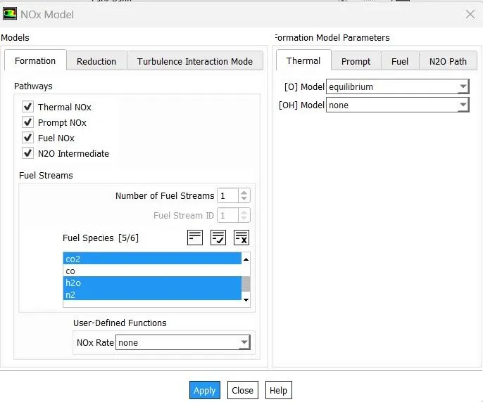
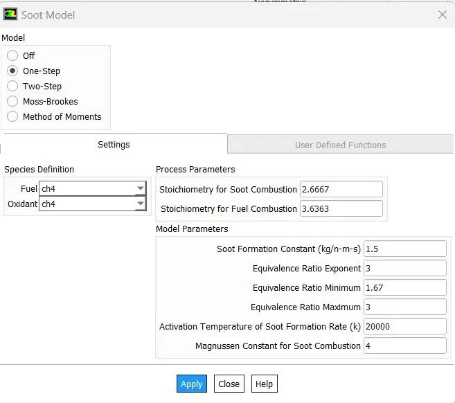
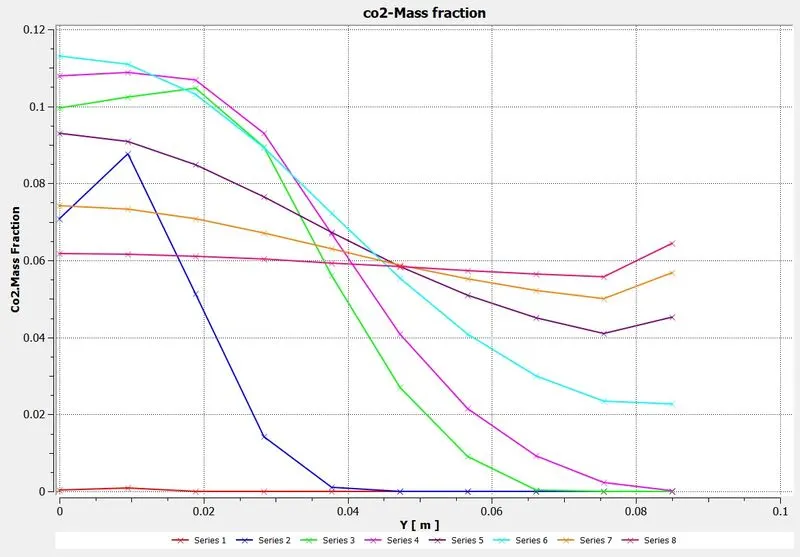
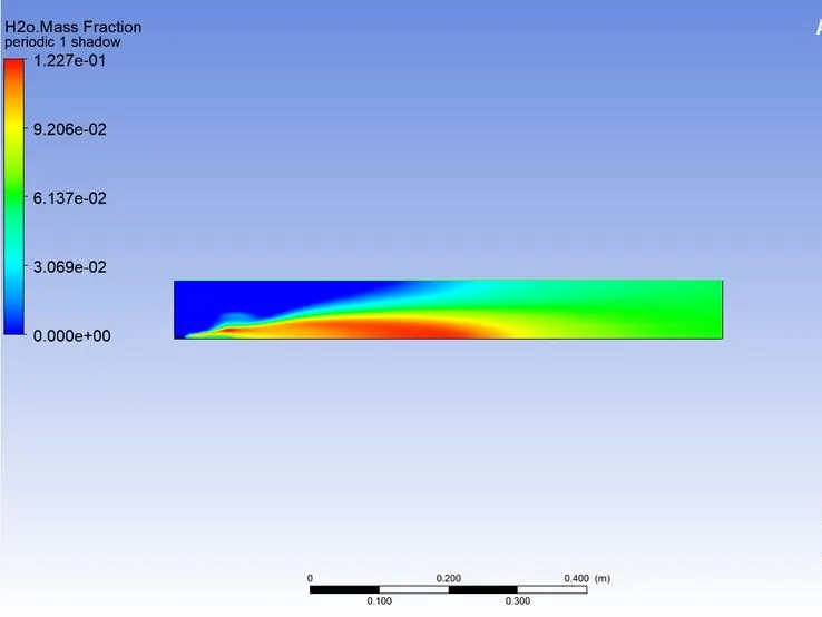
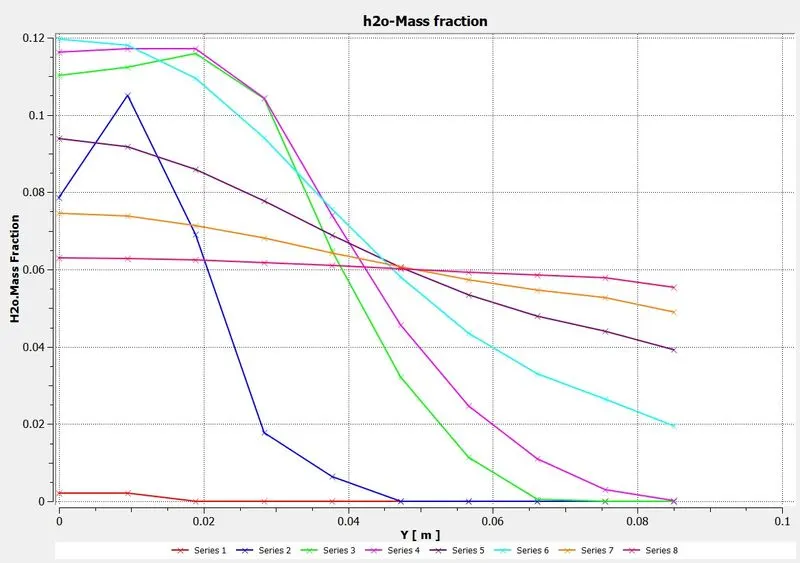
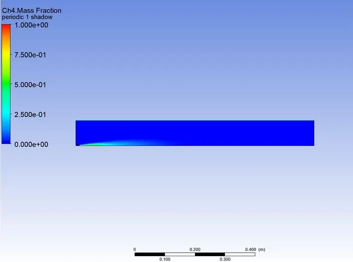
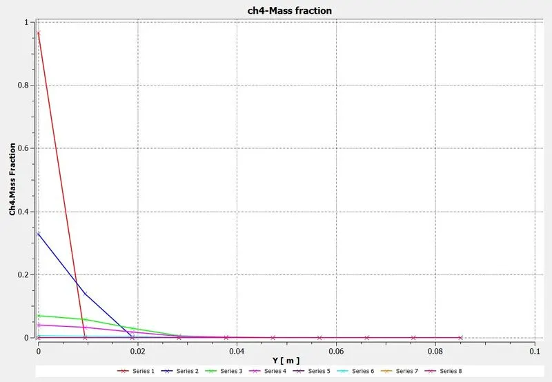
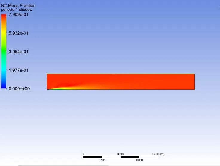
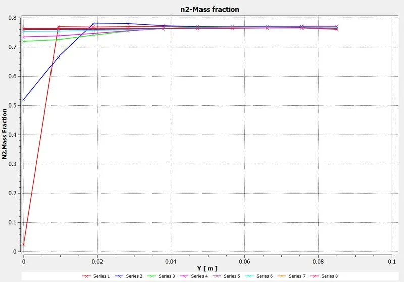
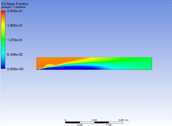
Perform a combustion simulation on the combustor model and plot the variation of the mass fraction of the different species’ in the simulation using line probes at different locations of the combustor as shown in Fig. You need to plot for CO2, H2O, CH4, N2, O2, NOx emissions & Soot formation.
Part II
As you must have observed from the above simulation, the Nox and soot is getting formed at the outlet of the combustor. Such formation has harmful effects on the environment and humans. The stringent government norms also demand the least formation of Nox and soot and to satisfy those requirements, you need to check the effect of adding the water in the fuel.
In this part, you need to add the water content in the fuel from 5% to 30% by mole and observe the effect of it on the results. It is necessary to provide line plots and contours to prove your claim.
Introduction:
Combustion:
A combustion is the Exothermic chemical reaction of a fuel with an oxidant to form the product. Basically there are two type combustion one is flame mode in which the thin zone of intense chemical reaction called ‘flame’ exist and another one is Non-flame mode in which volumetric combustion process is exited. The combustion simulation is performed to get the predictions of:
- flow fields and mixing characteristics
- Temperature fields
- Species Concentrations
- Particulates and pollutants.
The application of combustion modelling is applying for various kind of reacting flows such as furnaces, boilers, Process heaters, Gas turbines, automobiles and Rocket engines.
Modelling of combustion reaction in a software is difficult and need to take care for species which are taking part in reaction and its products. The combustion CFD model comprises of chemical kinetics and similarly achieving reacting flow mixture environment. Considering chemical kinetics, it is also important to have properly defined physical model with simulation to get the maximum out of process. Computational fluid dynamics of combustion model should be capable of enough to provide information related to species concentration, their volumetric generation or diffusion rate and changes in the system parameters like enthalpy, temperature and mixture density. The similar model should be good enough to solve the general transport equations for fluid flows and heat transfer as well as additional equations of combustion chemistry and chemical kinetics incorporated as per simulation environment details.
Chemical kinetics is part of combustion phenomenon, which is the study of entire reaction mechanism subject to different operating conditions. The whole reaction mechanism is the overall reaction of fuel and air with the elementary reaction. The elementary reaction is consisting of intermediate reaction cause generation of intermediate species, and the species react with fuel and air will cause the elementary reaction. This intermediate reaction caused due to breakup of chain reaction of fuel and air. The chemical kinetics is important as it provide when combustion process is going to start i.e. time period of ignition delay, rate of work done and used to determine emission from the chemical reactions. The elementary reactions in the case any combustion phenomena are mostly of three types which are bimolecular reactions, unimolecular reactions and termolecular reactions. In bimolecular reaction the reactants produce the product and same product can be undergoing to produce the reactant. This reaction is most common in combustion. In unimolecular reaction there are two types one is isomerization in which transformation of composition is occurred and another case is decomposition in which breakdown of composition is occurred.
Based on mixing:
Premixed combustion:
- In the mixing chamber, fuel and oxidizer (air) are already mixed at the molecular level before ignition or combustion
- Cold reactants propagate into hot products
- Rate of propagation (flame speed) depends on the internal flame structure
- Much more difficult to model than non-premixed combustion problems
- Turbulence distorts the laminar
- Examples: SI engine, LPG gas stove etc.
Non-premixed combustion:
- Separate inlet/ streams for Fuel and oxidizer (air) to the combustion chamber
- Convection or diffusion of reactants from either side into a flame sheet
- Turbulent eddies distort the laminar flame shape and enhance mixing
- May be simplified to a mixing problem
- Examples: Burner for boiler /furnaces, coal combustion, candle flame, wood fire etc.
Partially premixed combustion:
- In some applications, primary air (oxidizer) is mixed with fuel to form the unburnt mixture before combustion such cases are treated as partially premixed combustion.
- Premixed fuel/oxidizer inlet streams
Based on Phase:
Volumetric: Takes place when the fluid is in fluid phase.
Surface: Takes place on the wall.
Porous: Takes place inside pores
Eddy dissipation:
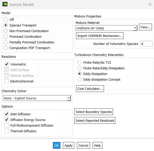
Most fuels are fast burning and the overall rate of reaction is controlled by turbulence mixing. In the non-premixed flames, turbulence slowly mixes the fuel and oxidizer into the reaction zones where they burn quickly. In premixed flames the turbulence slowly mixes cold reactants and hot products into the reaction zones where reaction occurs rapidly. In such cases the combustion is said to be mixing-limited, and the complex and often unknown chemical kinetics can be safely neglected. In this model, the chemical reaction is governed by large eddy mixing time scale. Combustion initiates whenever there is turbulence present in the flow. It does not need an ignition source to initiate the combustion. This type of model is valid for the non-premixed combustion, but for the premixed flames the reactant is assumed to burn at the moment it enters the computation model, which is a shortcoming of this model as in practice the reactant needs some time to get to the ignition temperature to initiate the combustion.
Pre-processing
Space claim:
- Importing CAD file into Ansys Space Claim: Open Ansys ⇒ Geometry ⇒ drag and drop the file.
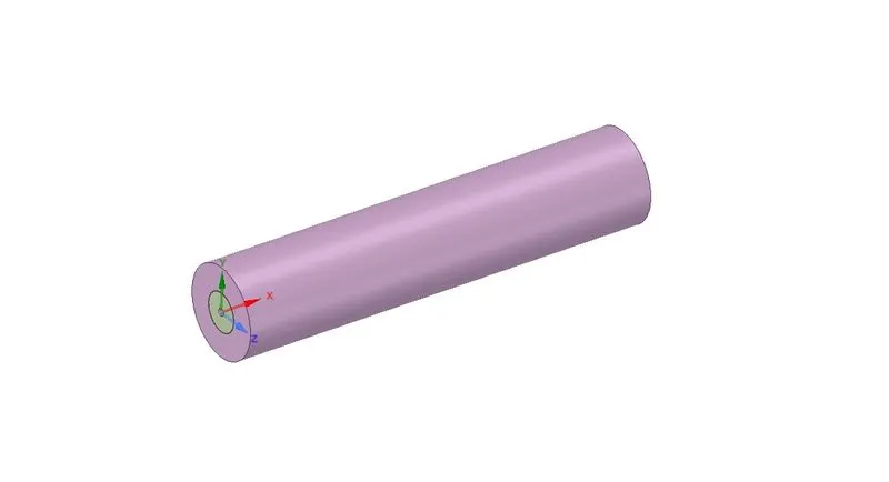
3D model will increase the computational cost and time to run the simulation and also in an Academic license there are limitations for mesh generation. So we are extracting the 2D model from the 3D model and doing a simulation on it.
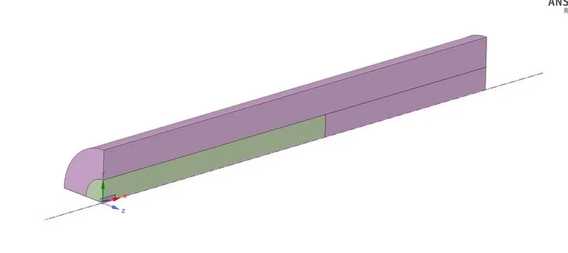

Meshing:
Naming and Meshing:
Axis:
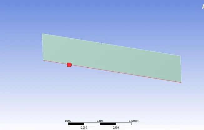
Fuel Inlet:
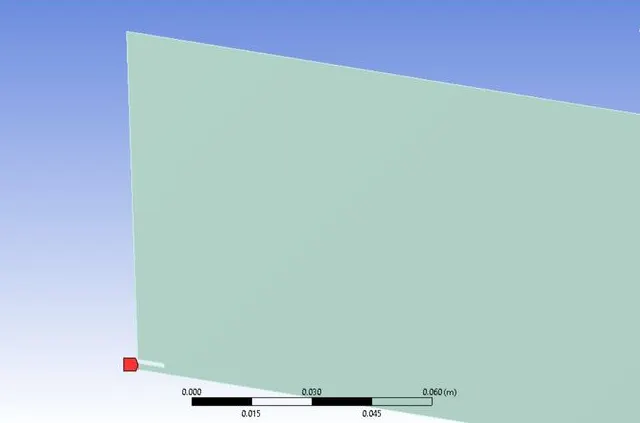
Air Inlet:
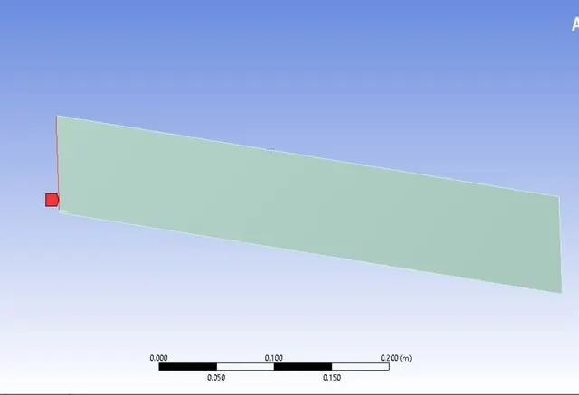
Outlet:
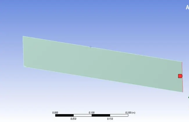
Wall:
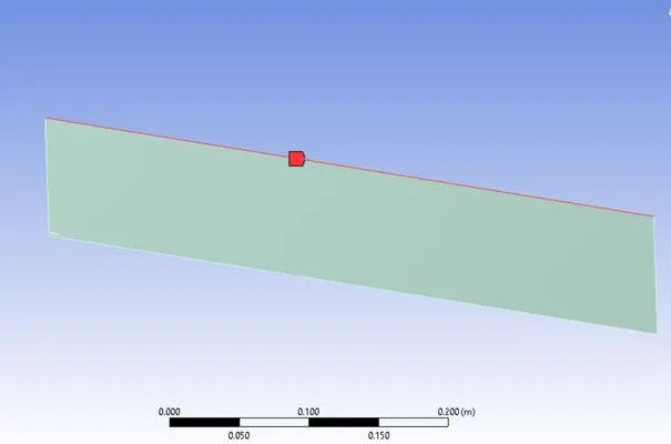
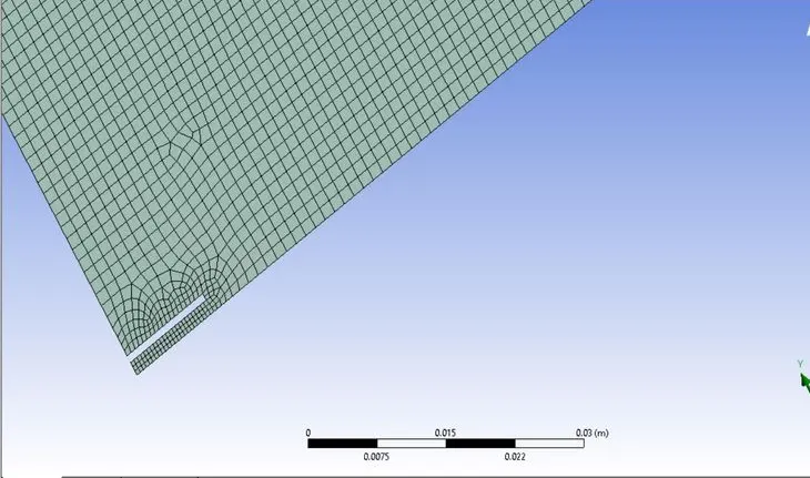
Mesh:
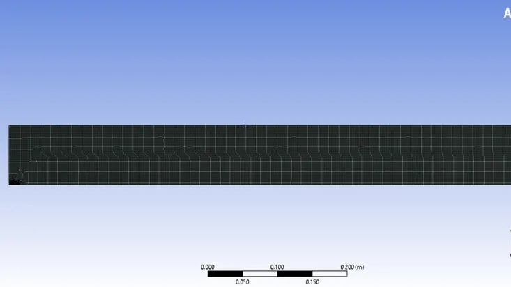
For refining the mesh for this case we are using the all triangle method.
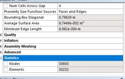
- Element size = 0.15 mm
- Capture proximity ON
- Proximity minimum size = 0.025 mm
- Number of cells across gap = 4
- Number of Nodes = 30850
- Number of Elements = 30232
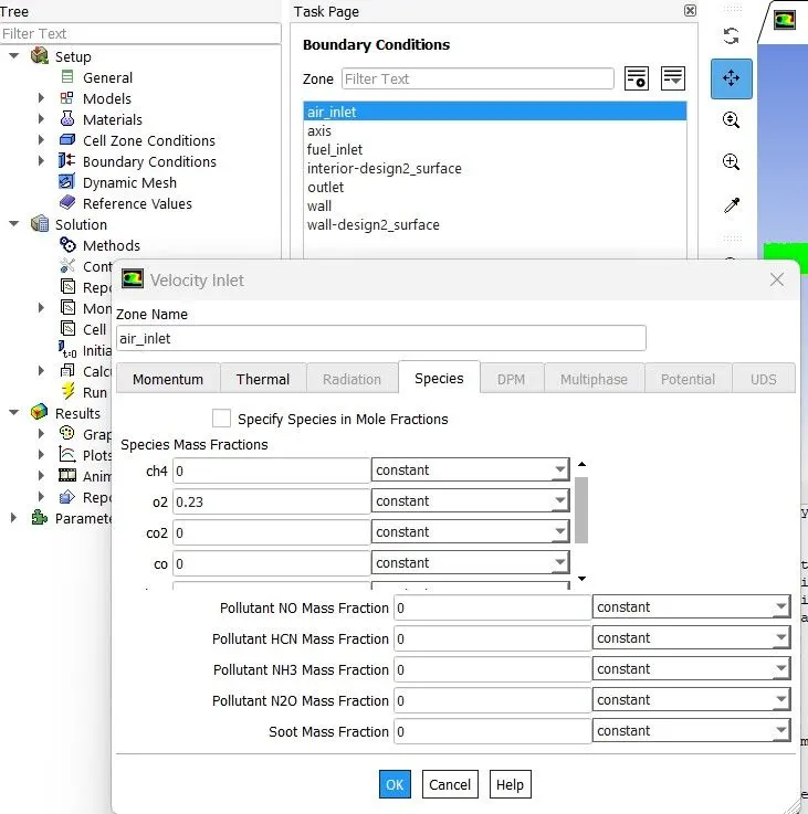
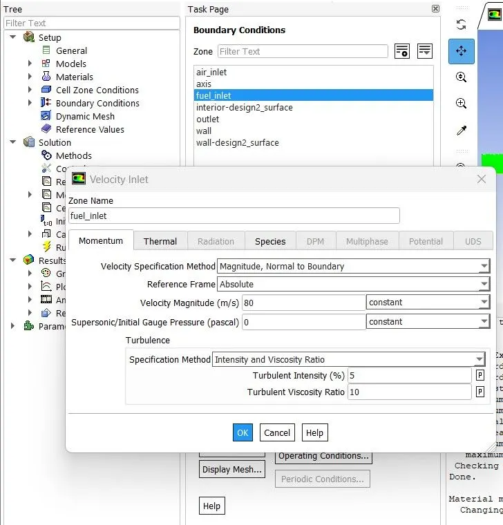
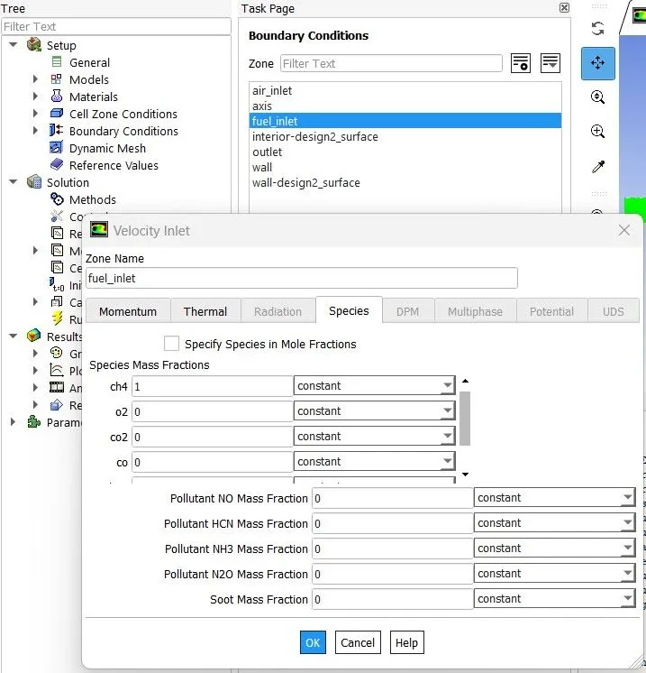
Setting up physics and Boundary conditions:
Setup:
|
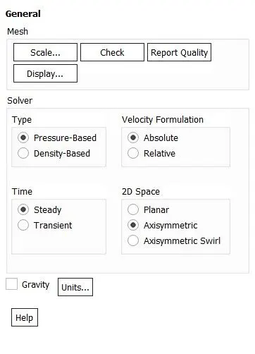
Solver Type |
Pressure-Based |
|
Velocity Formulation |
Absolute |
|
2D Space |
Axisymmetric |
|
Time |
Steady State |
|
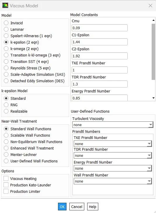
Viscous Model |
K-epsilon > Standard > Scalable wall Function Energy - On |
|
Models |
Species > Species Transport - On |
|
Material |
Fluid Type - Air Solid Type - Aluminum Mixture - Methane-air-2step |
|
Boundary Condition |
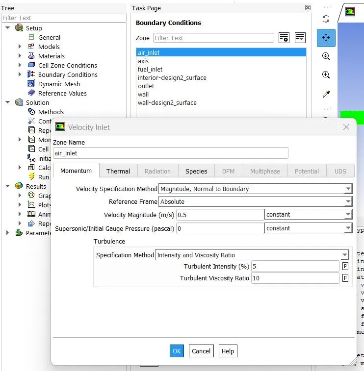
Air Inlet - Fuel Inlet - |
|
) as per cases Outlet - Pressure outlet (Gauge pressure = 0 Pa) Walls - Stationary wall with no-slip condition Axis - Axisymmetric (x-axis) |
|
|
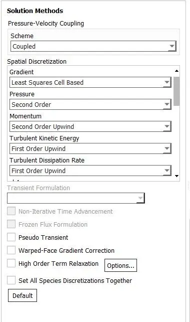
Solution Method |
pressure-velocity coupling- COUPLED |
|
Initialization |
Standard Initialization |
Result:
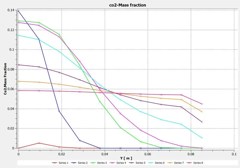
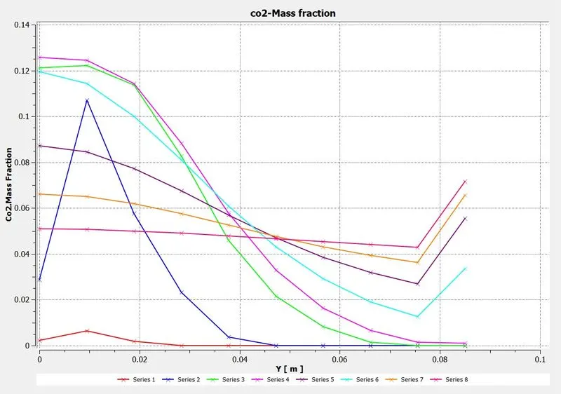
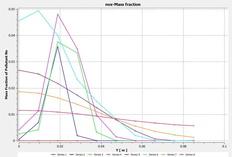
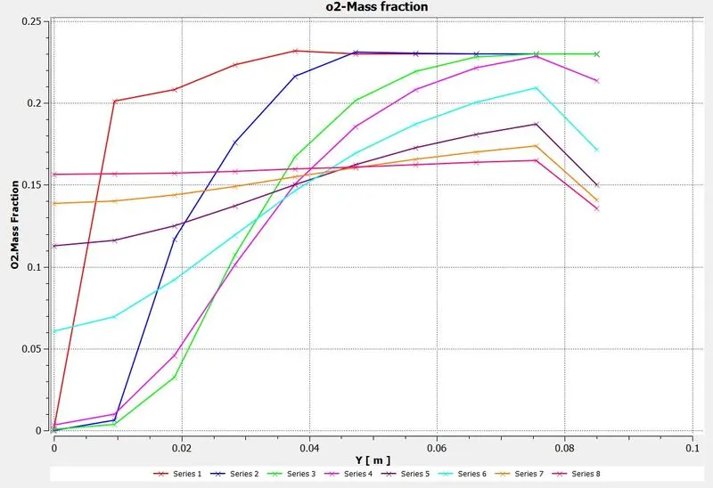
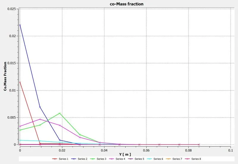
Coordinates of Line probes :
Line 1 :
Point 1---> x=0.015m y=0m z=0m
Point 2---> x=0.015m y=0.085m z=0m
Line 2 :
Point 1---> x=0.1m y=0m z=0m
Point 2---> x=0.1m y=0.085m z=0m
Line 3 :
Point 1---> x=0.25m y=0m z=0m
Point 2---> x=0.25m y=0.085m z=0m
Line 4 :
Point 1---> x=0.3m y=0m z=0m
Point 2---> x=0.3m y=0.085m z=0m
Line 5 :
Point 1---> x=0.4m y=0m z=0m
Point 2---> x=0.4m y=0.085m z=0m
Line 6 :
Point 1---> x=0.5m y=0m z=0m
Point 2---> x=0.5m y=0.085m z=0m
Line 7 :
Point 1---> x=0.6m y=0m z=0m
Point 2---> x=0.6m y=0.085m z=0m
Line 8 :
Point 1---> x=0.79m y=0m z=0m
Point 2---> x=0.79m y=0.085m z=0m
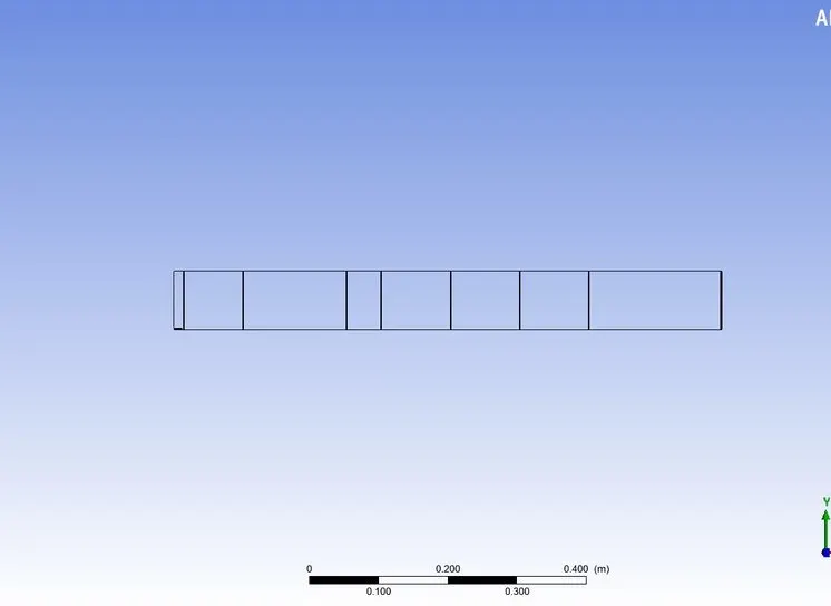
Result:
Case 1-
Mole Fraction - ch4 =1 ; h2o = 0
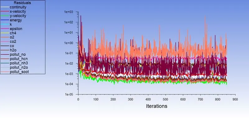
Residual Plot:
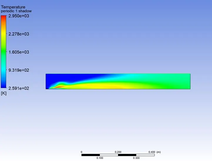
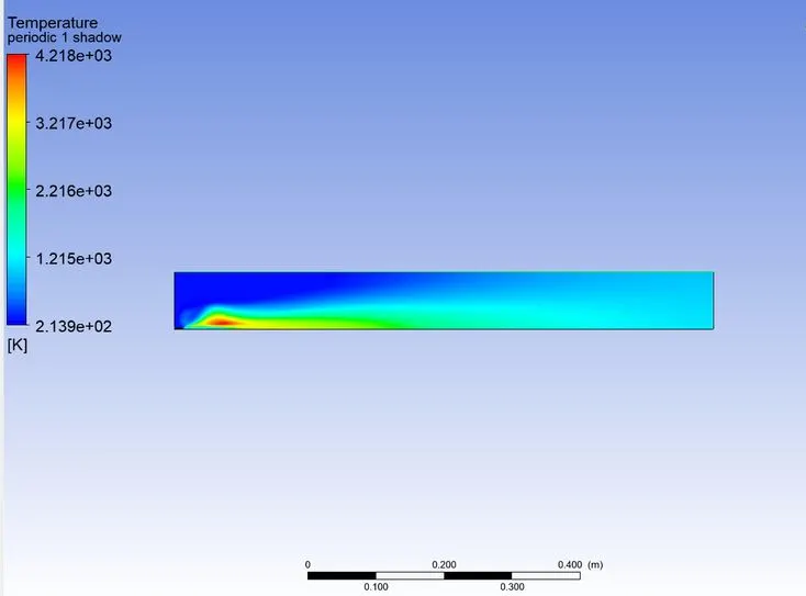
Temperature contour:
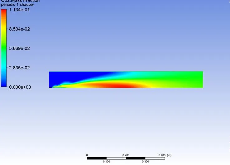
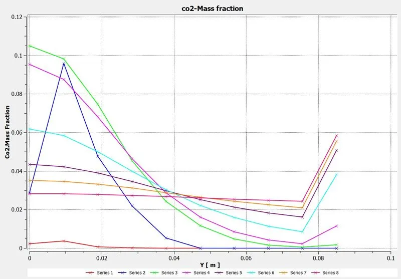
Contour and plot of co2 mass fraction:
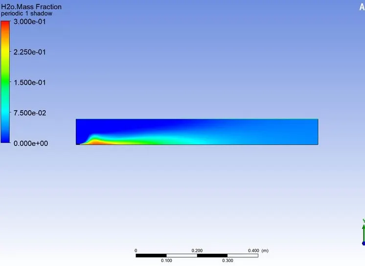
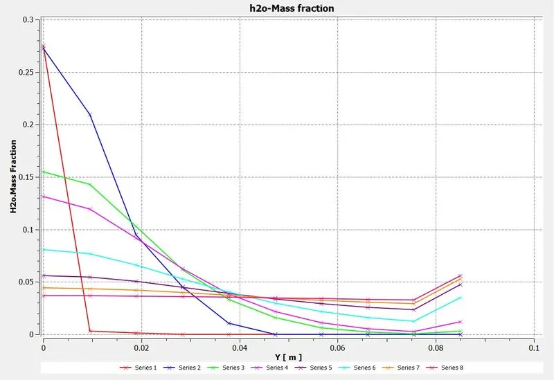
Contour and plot of h2o mass fraction:
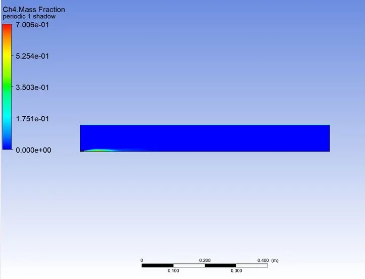
Contour and plot of ch4 mass fraction:
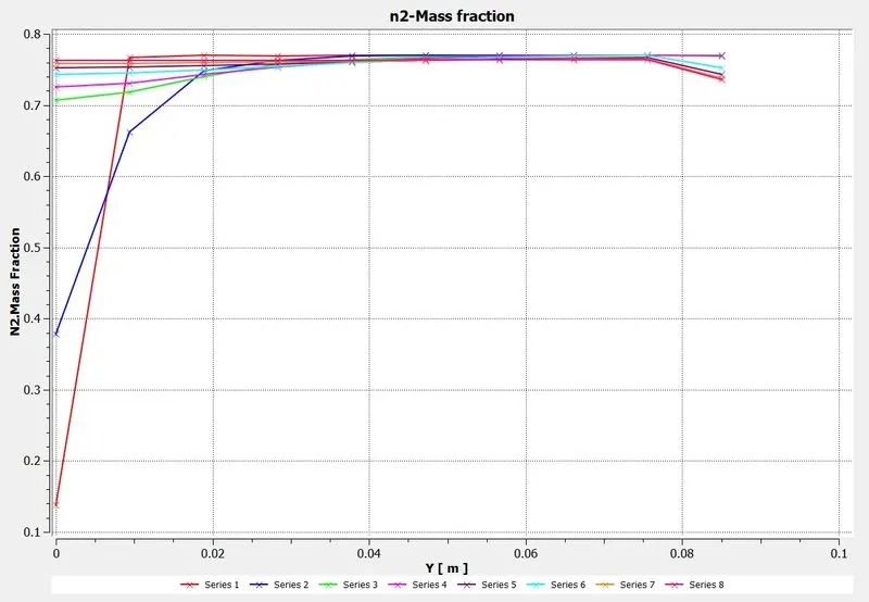
Contour and plot of N2 mass fraction:
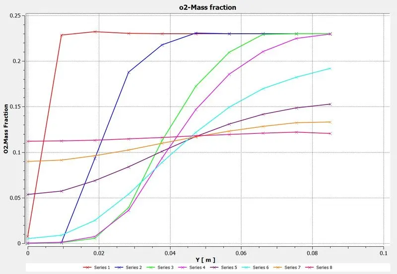
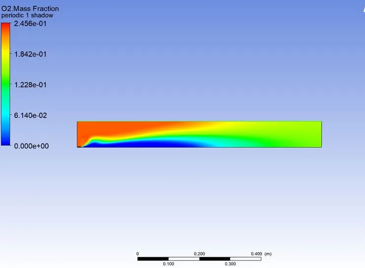
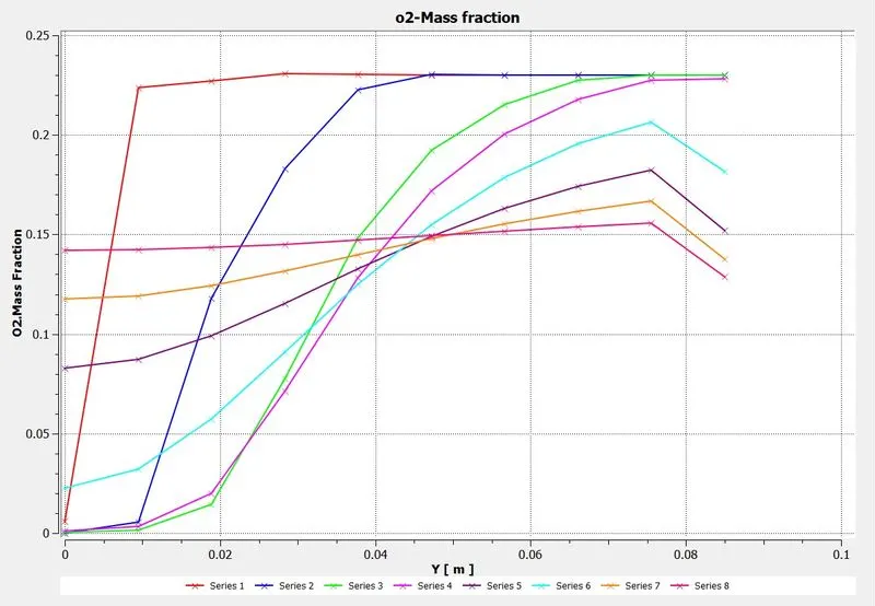
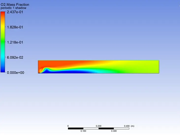
Contour and plot of o2 mass fraction:
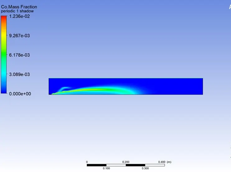
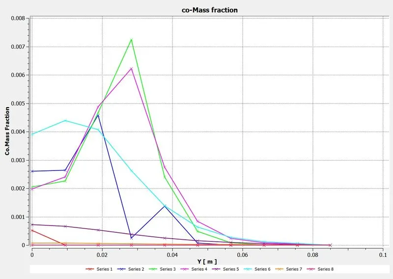
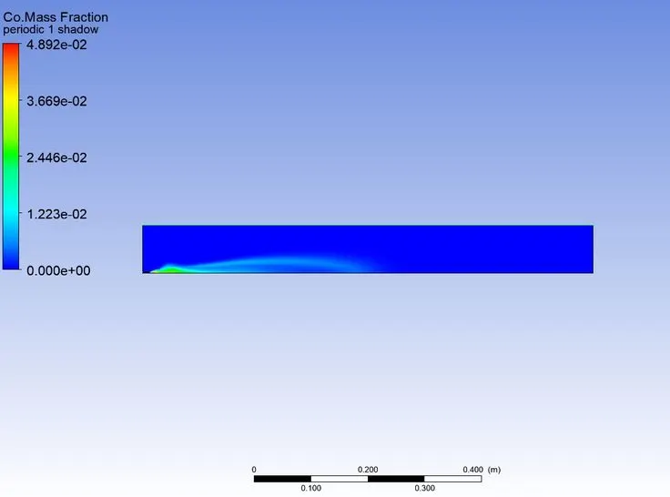
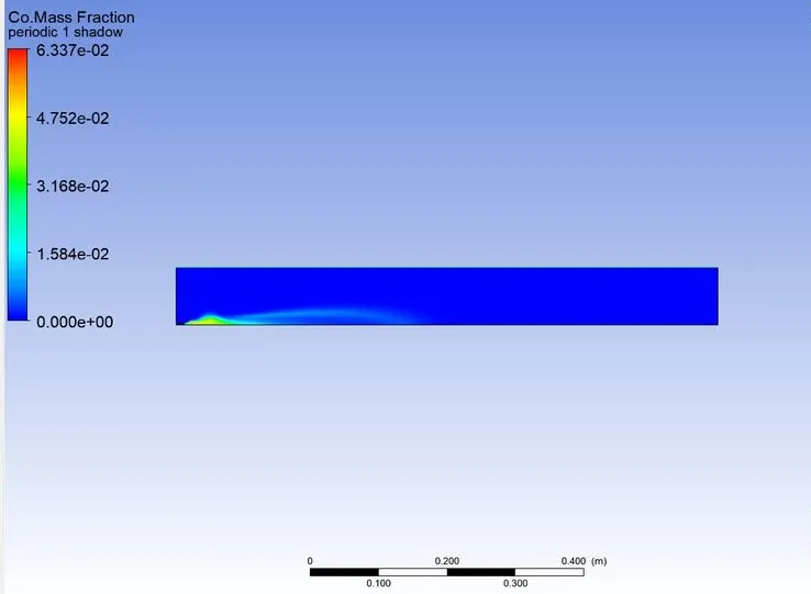
Contour and plot of co mass fraction:
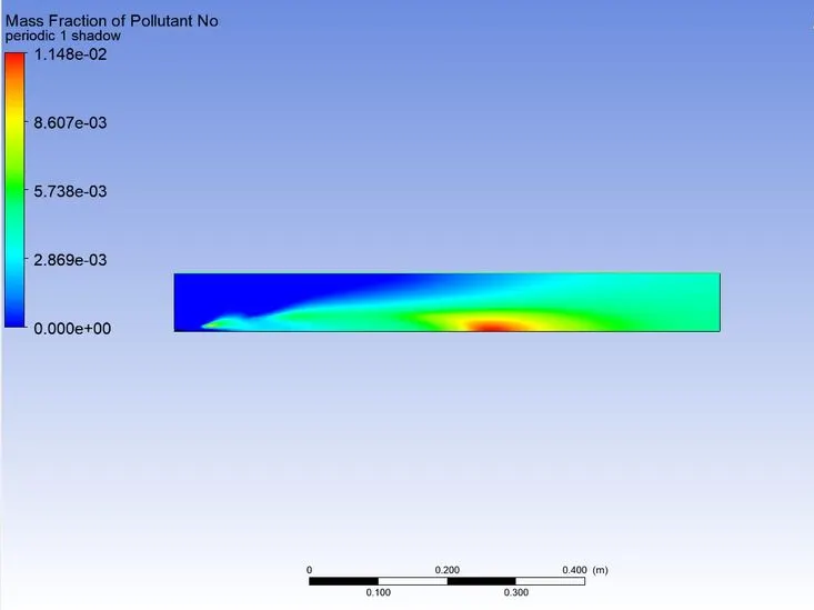
Contour and plot of nox mass fraction:
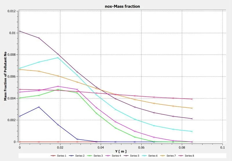
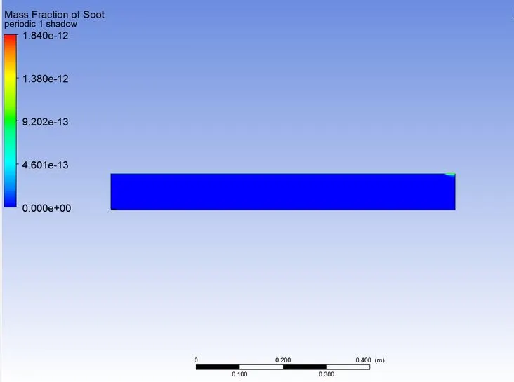
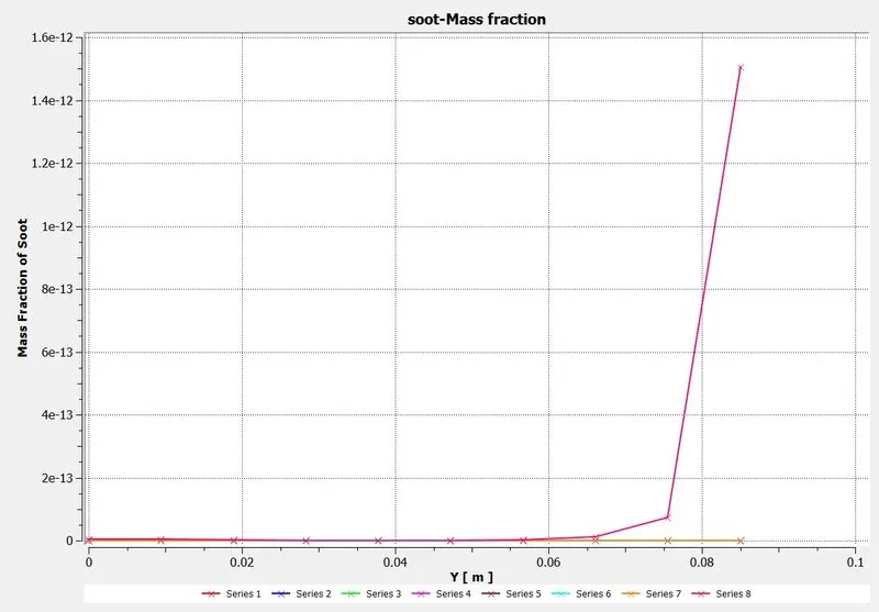
Contour and plot of soot mass fraction:
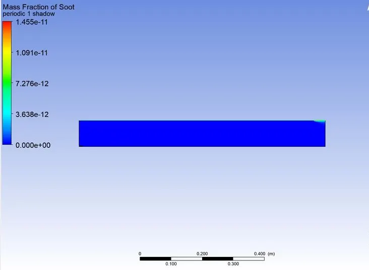
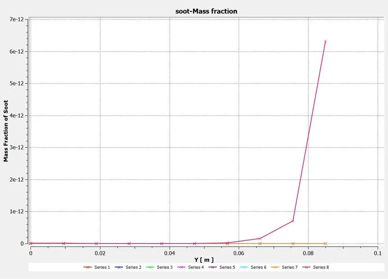
Case 2-
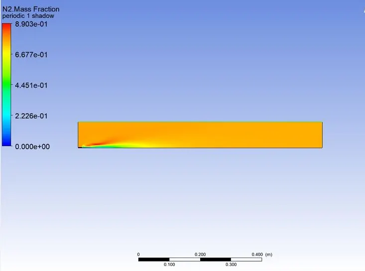
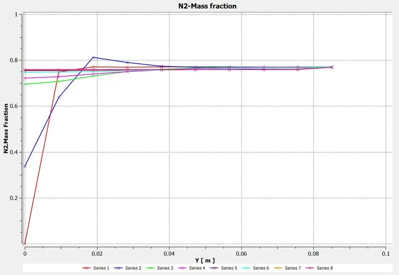
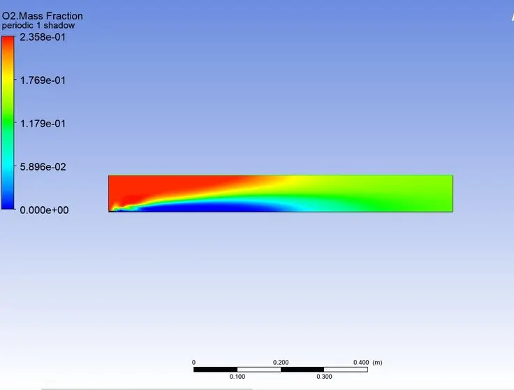
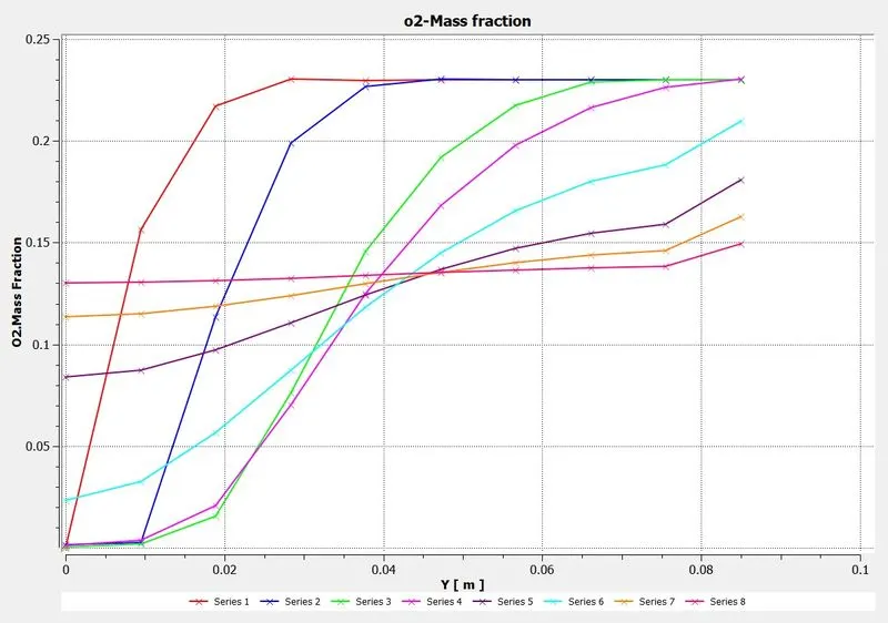
Mole Fraction - ch4 =0.95 ; h2o = 0.05 :
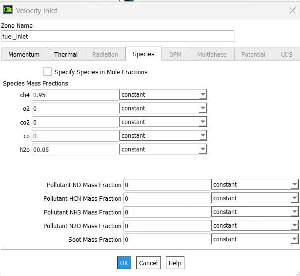
Result:
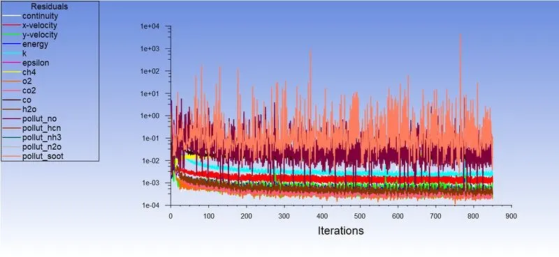
Residual Plot:
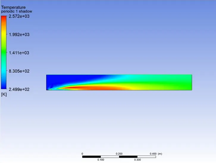
Temperature Contour:
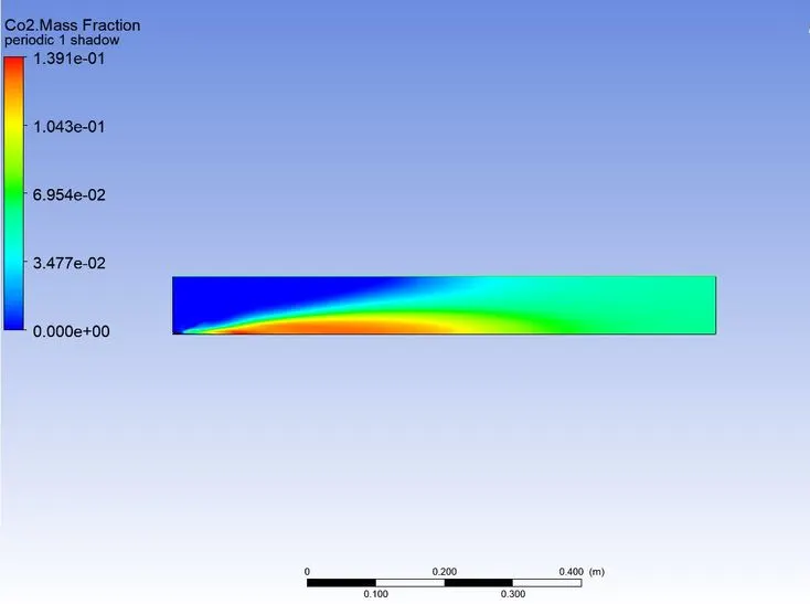
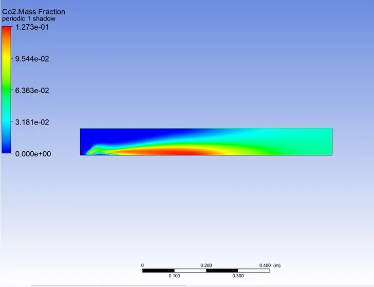
Contour and plot of co2 mass fraction:
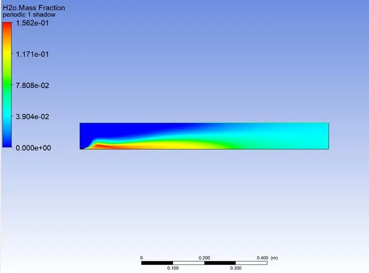
Contour and plot of h2o mass fraction:
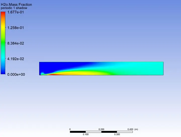
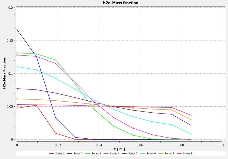
Contour and plot of ch4 mass fraction:
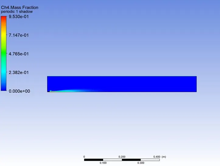
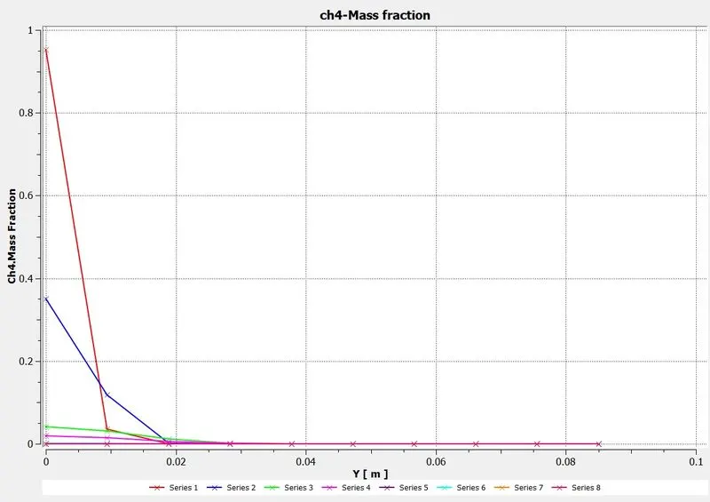
Contour and plot of N2 mass fraction:
Contour and plot of o2 mass fraction:
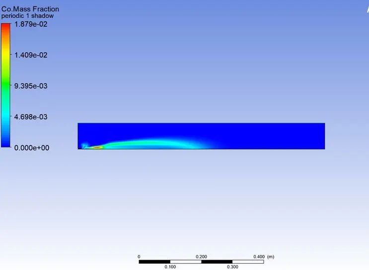
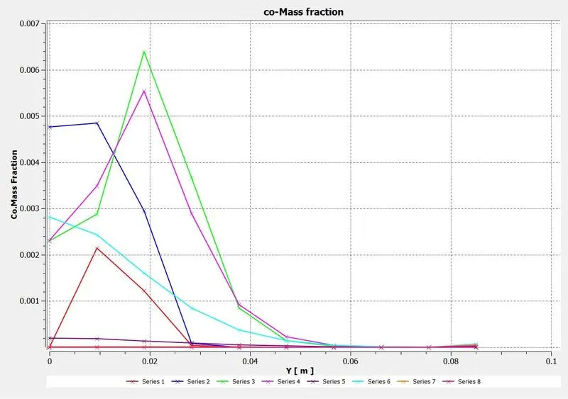
Contour and plot of co mass fraction:
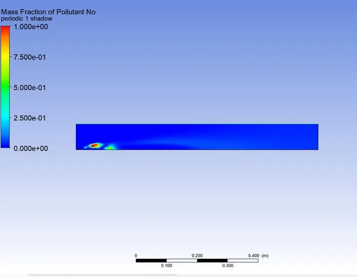
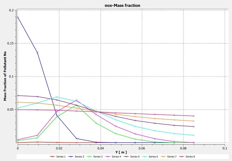
Contour and plot of nox mass fraction:
Contour and plot of soot mass fraction:
Case 3-
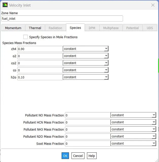
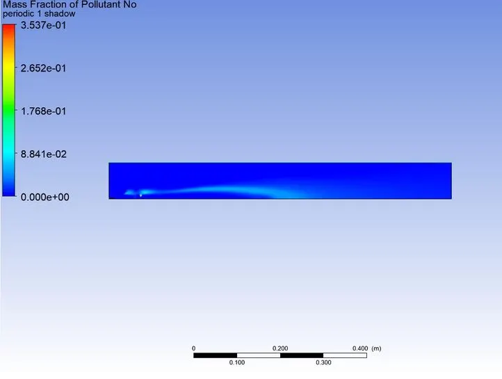
Mole Fraction - ch4 =0.9 ; h2o = 0.1:
Result:
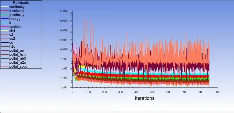
Residual Plot:
Temperature Contour:
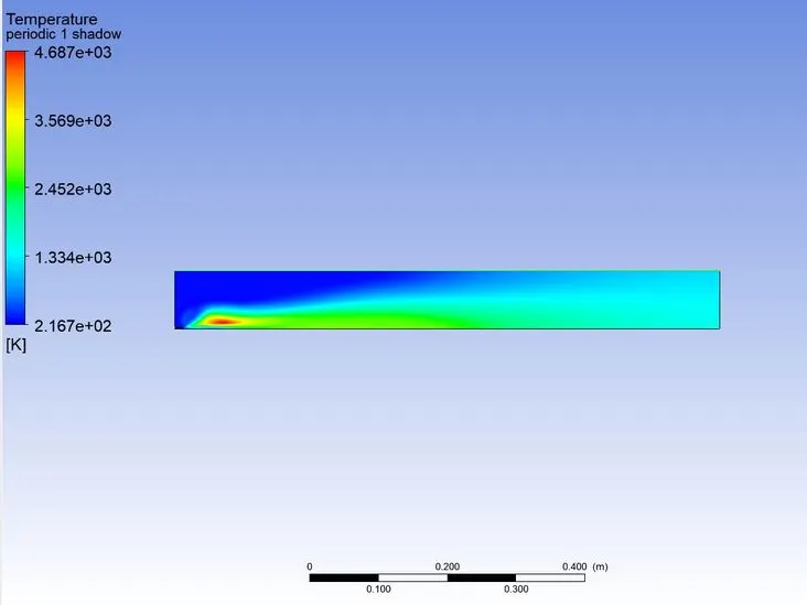
Contour and plot of co2 mass fraction:
Contour and plot of h2o mass fraction:
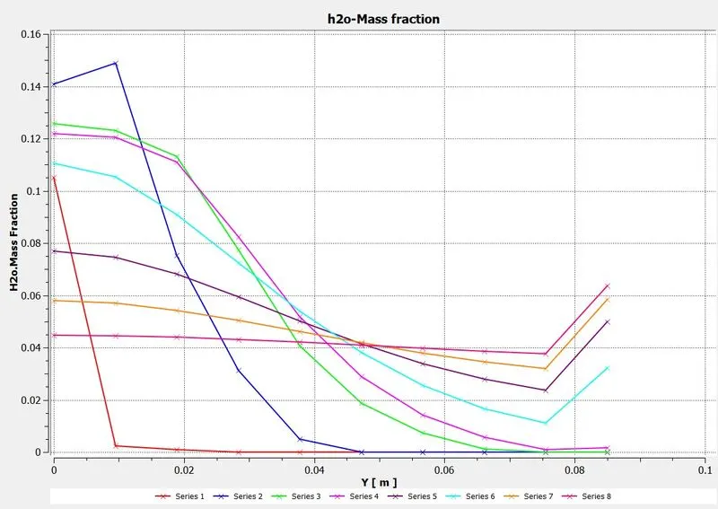
Contour and plot of ch4 mass fraction:
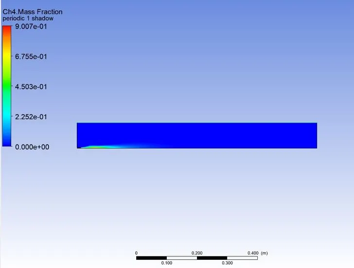
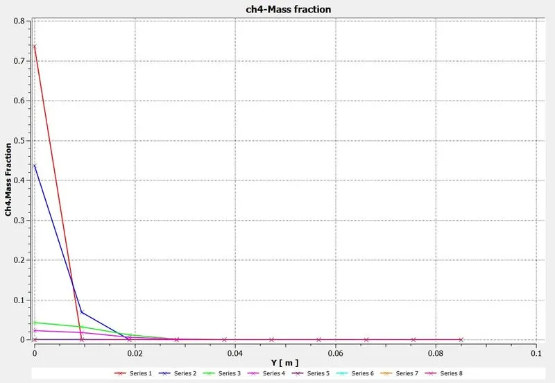
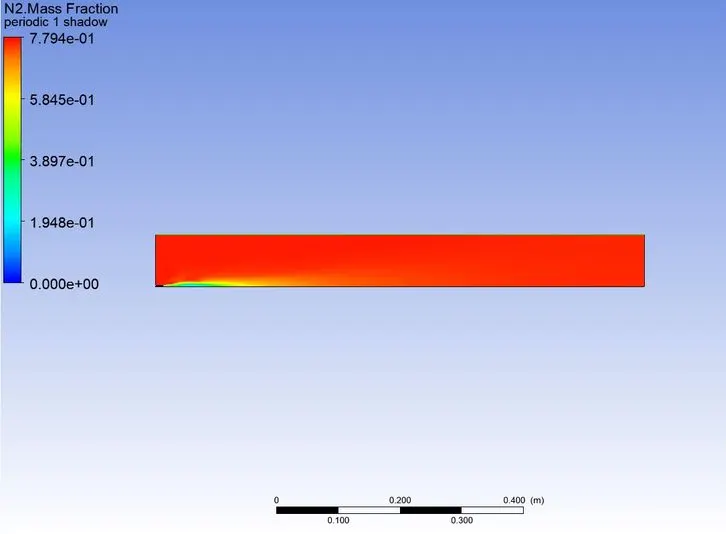
Contour and plot of N2 mass fraction:
Contour and plot of o2 mass fraction:
Contour and plot of co mass fraction:
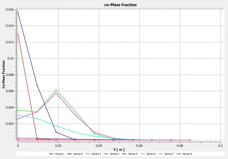
Contour and plot of nox mass fraction:
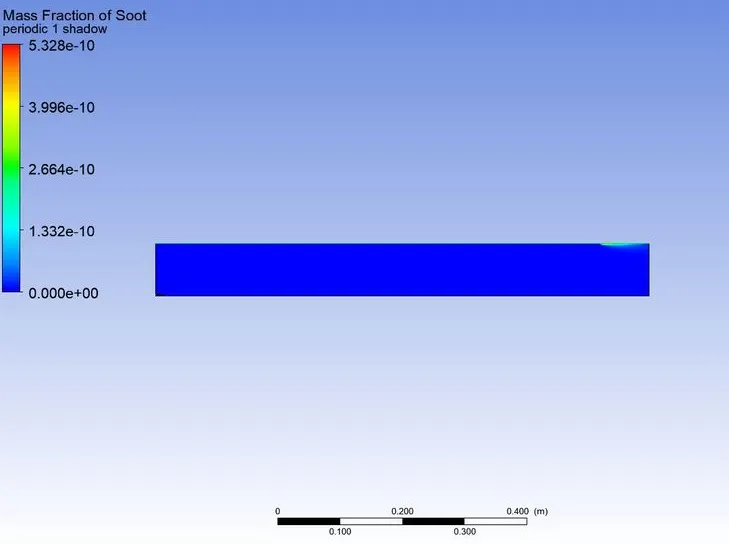
Contour and plot of soot mass fraction:
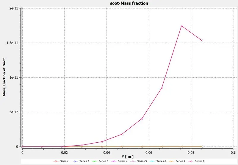
Case 4-
Mole Fraction - ch4 =0.8 ; h2o = 0.2:
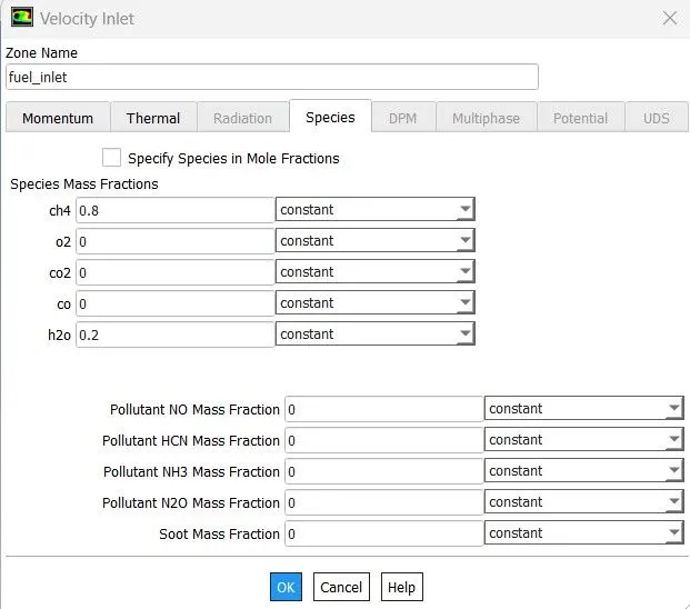
Result:
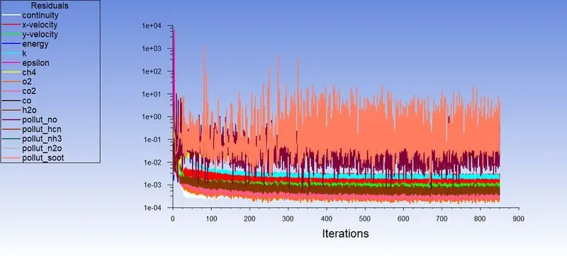
Residual Plot:
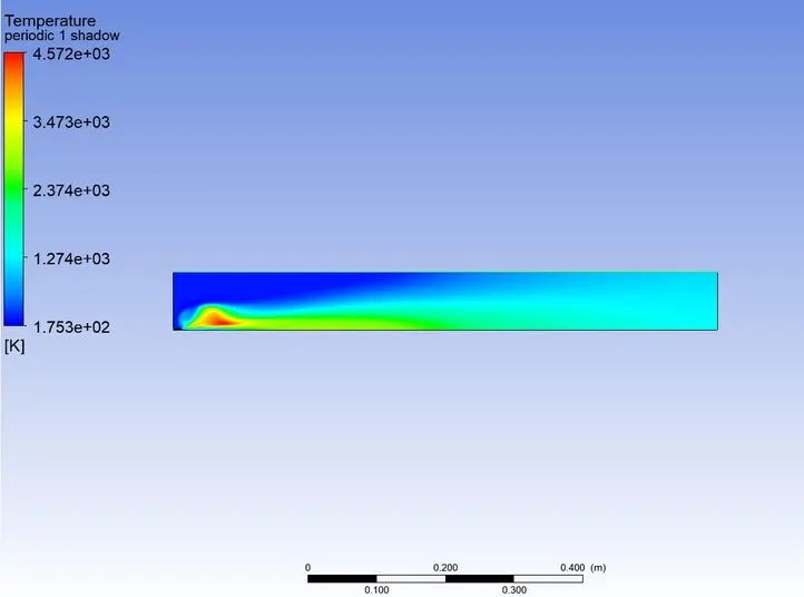
Temperature Contour:
Contour and plot of co2 mass fraction:
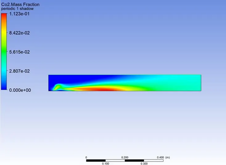
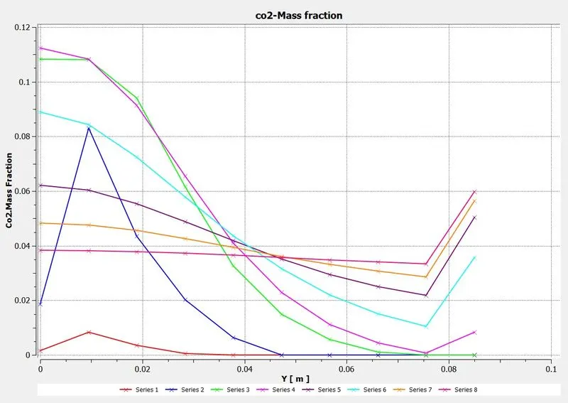
Contour and plot of h2o mass fraction:
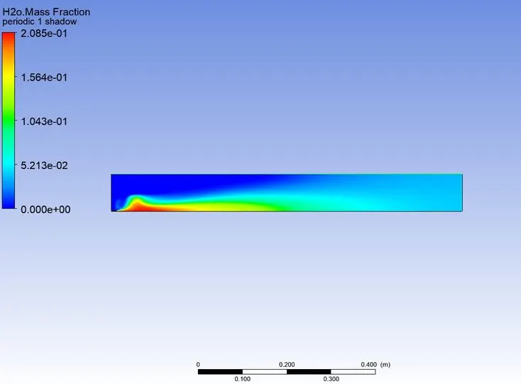
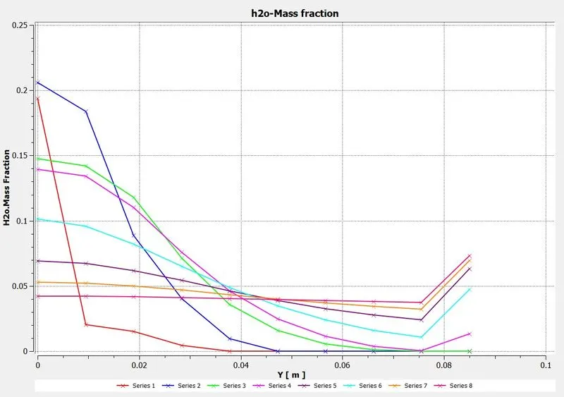
Contour and plot of ch4 mass fraction:
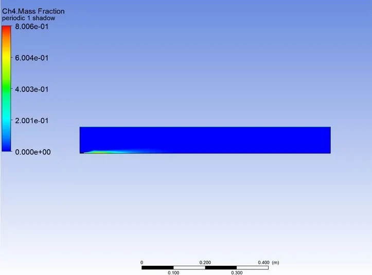
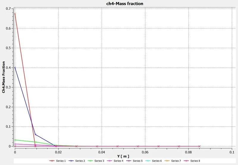
Contour and plot of N2 mass fraction:
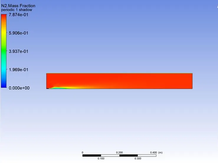
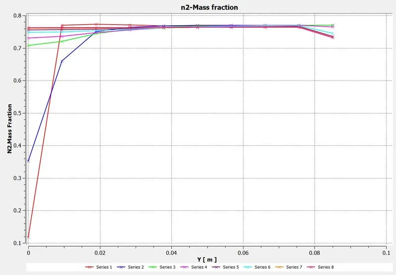
Contour and plot of o2 mass fraction:
Contour and plot of co mass fraction:
Contour and plot of nox mass fraction:
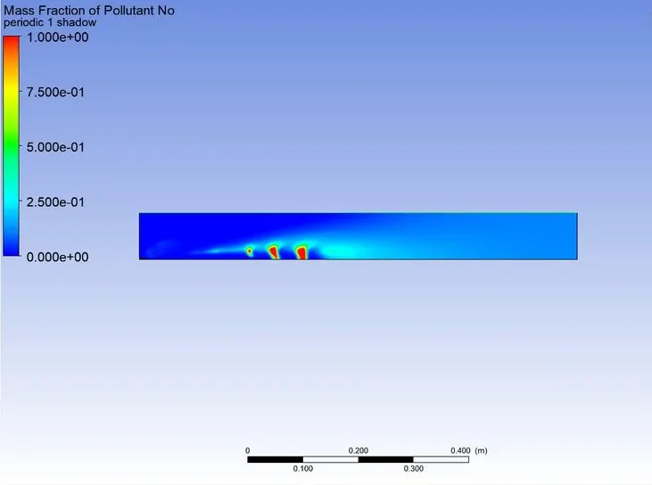
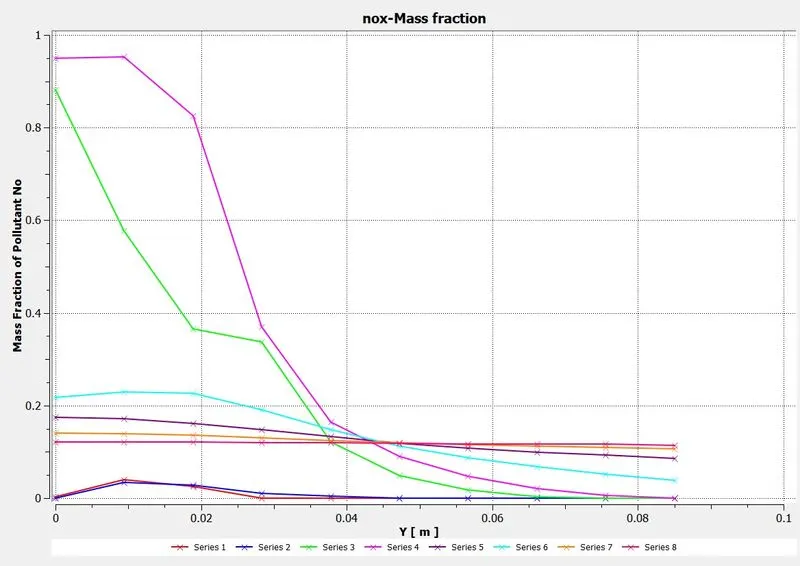
Contour and plot of soot mass fraction:
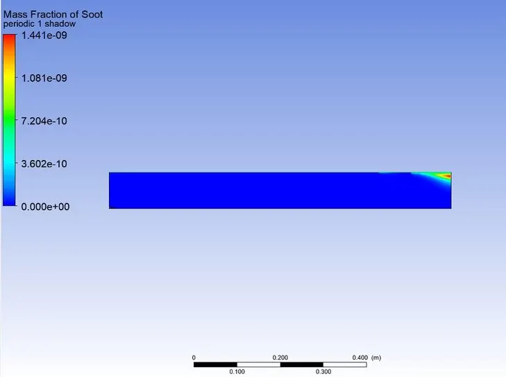
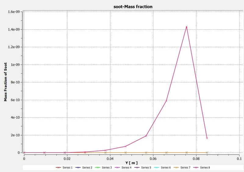
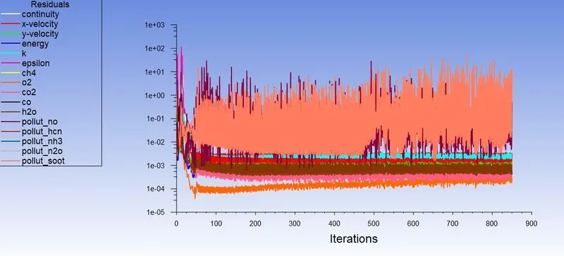
Case 5-
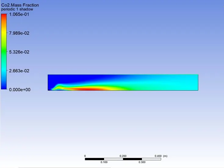
Mole Fraction - ch4 =0.7 ; h2o = 0.3:
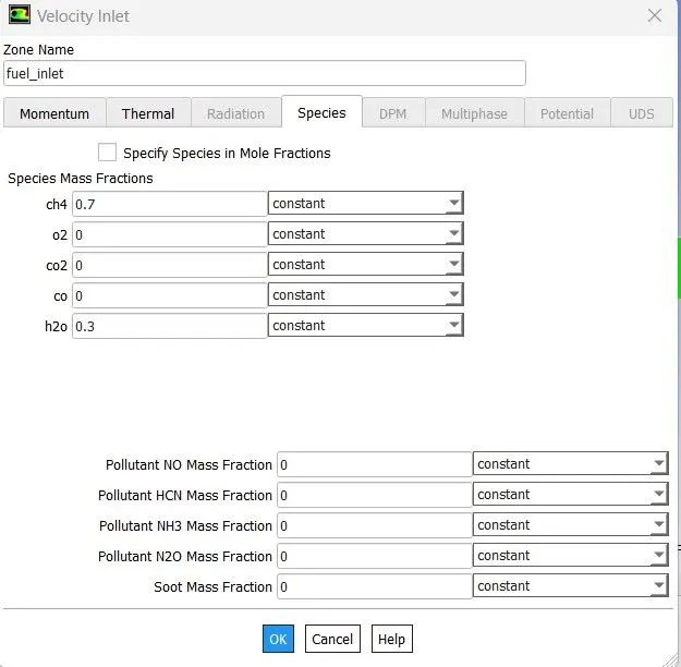
Result:
Residual Plot:
Temperature Contour:
Contour and plot of co2 mass fraction:
Contour and plot of h2o mass fraction:
Contour and plot of ch4 mass fraction:
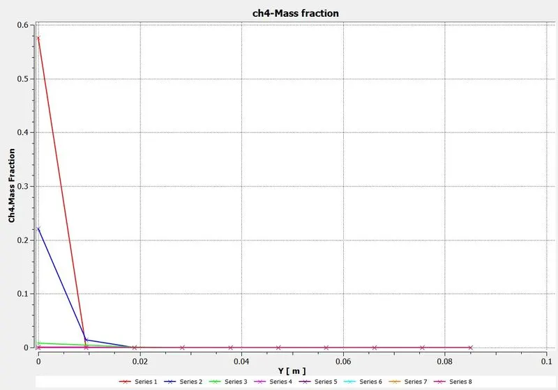
Contour and plot of N2 mass fraction:
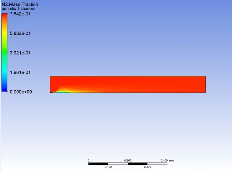
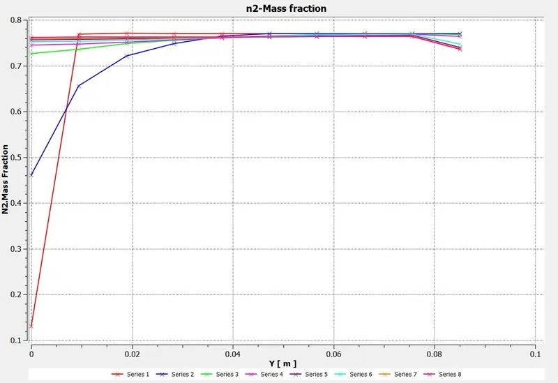
Contour and plot of o2 mass fraction:
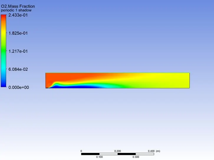
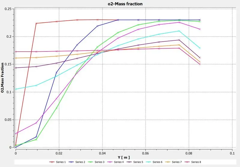
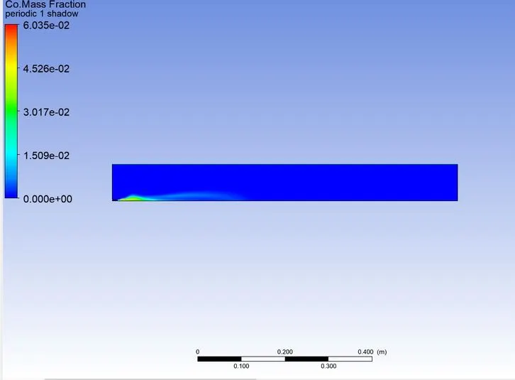
Contour and plot of co mass fraction:
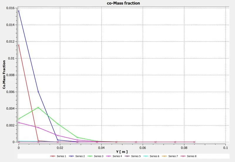
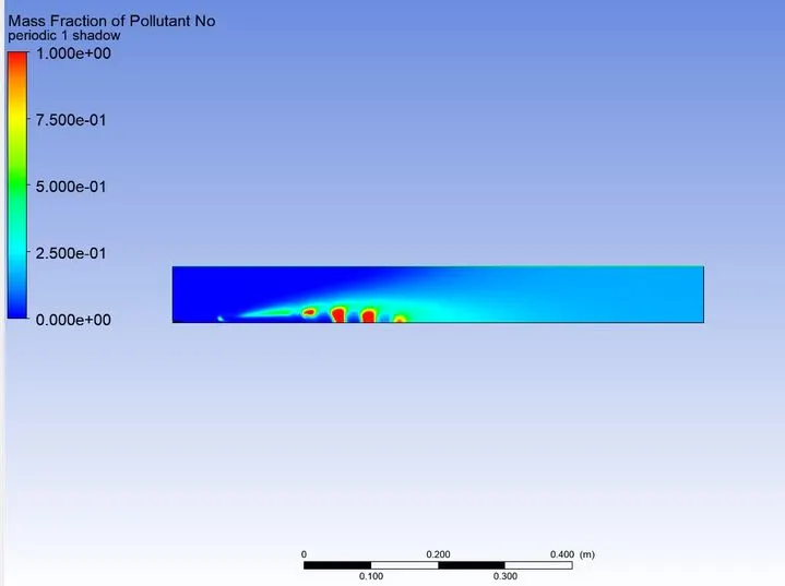
Contour and plot of nox mass fraction:
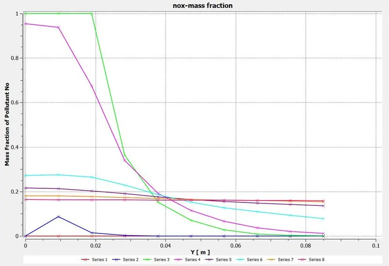
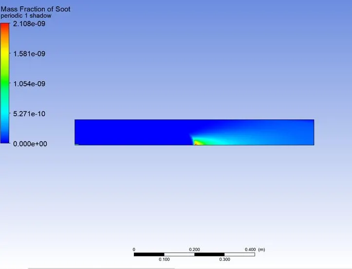
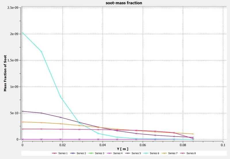
Contour and plot of soot mass fraction:
Inference:
Result Table:
| Parameter | Baseline Mesh | Case 1 - 5% oxygen | Case 2 - 10% oxygen | Case 3 - 20% oxygen | Case 4 - 30% oxygen |
| Mass Fraction of ch4 | 1 | 0.95 | 0.9 | 0.8 | 0.7 |
| Mass Fraction of o2 | 0.2539 | 0.2358 | 0.2455 | 0.2436 | 0.2433 |
| Mass Fraction of co2 | 0.1133 | 0.139 | 0.1272 | 0.1122 | 0.1063 |
| Mass Fraction of co | 0.0123 | 0.0189 | 0.0489 | 0.0633 | 0.0603 |
| Mass Fraction of h2o | 0.1227 | 0.1676 | 0.1561 | 0.2085 | 0.3 |
| Mass Fraction of n2 | 0.7908 | 0.8902 | 0.7793 | 0.7874 | 0.7842 |
| Mass Fraction of NOX | 0.0114 | 1 | 0.3536 | 1 | 1 |
| Mass Fraction of soot | 1.45 e-11 | 1.84 e-12 | 5.32 e-10 | 1.44 e-09 | 2.10 e-09 |
Conclusion:-
- Diluting fuel with H2O">H2O does indeed reduce the formation of harmful pollutants such as NOX">
- and soot at the outlet.
- The rate of reduction in the concentration of soot is greater than that of NOX">
- when diluting the fuel with water.
- Addition of water is also lead to decrease in temperature of combustor
- Fuel dilution by H2O">
- is a great way to reduce emissions. However, a trade-off must be made between the performance required and the dilution amount.
- Since soot value decreases with dilution we can say there is less wastage of fuel, i.e. complete combustion occurs.
- Eddy - dissipation model(Turbulence Chemistry Interaction) helps us to model combustion via turbulence mixing without the presence of an ignition source.